How To Use Python
 python.org
1 Introduction
As a bioinformatics researcher, I primarily use the statistical programming language R for my analyses, mainly due to the huge number of resources available in the Bioconductor libraries. I have previously written a Tutorial for R, so thought that I would do something similar for the data science programming language Python.
Python is an interpreted, high-level language that supports both object-oriented and structured programming. Both Python and R are widely used in the data science world, with both having very similar functionality, but specific pros and cons making the “correct” choice for which one to use being somewhat dependent on the task at hand. Python is typically considered to be more memory efficient than R, and has some amazingly powerful libraries for data science such as scikit-learn and TensorFlow, whilst R has amazing libraries for bioinformatics and superb data visualization through the ggplot2 package and the other TidyVerse packages from Hadley Wickham.
However, R has some amazingly memory-efficient implementations (including an interface to TensorFlow and other machine learning tools), and Python has a huge bioinformatics suite with the biopython suite and excellent plotting packages such as seaborn. So ultimately, both are excellent, and knowing either can be a fantastic tool in your data science toolbox.
This is an introduction to Python that should allow new users to understand how Python works. It will follow a similar flow to the R introduction, so the two can be compared to understand the differences between the two languages.
As with R and other languages, comments can be added using the # comment character. Everything to the right of this character is ignored by Python. This allows you to add words and descriptions to your code which are ignored entirely by the interpreter, but can be used for people looking at the source code to help document what a particular code chunk does. You can NEVER have too many comments!
2 Installing Python
Python can be downloaded and installed from the Python website. It is available for all major operating systems, and installation is quite straightforward. The current version is 3.8.0, but updates are released regularly. Additional packages can be installed by using the pip Python package manager as follows:
pip install newpackageIt is also possible to use larger package managers such as the Anaconda data science platform. This is an open-source distribution containing over 1,500 Python and R packages that ensures all dependencies are maintained and any required packages are present. conda will allow you to generate multiple environments to work in depending on requirements.
Unlike R, there is no specific Integrated Development Environment, but there are multiple different programs that can be sconsidered such as Spyder and PyCharm. There is also the Jupyter notebook program, which allows interactive computing supporting many different programming languages. This is similar to R markdown (which is used to generate the content of this blog), in that it merges markdown formatted text with code chunks. This can be used to create auto-generated reports by including code output embedded into the text.
3 Basics of Python
3.1 Getting started
If using a command line interface, Python can be run simply by typing the name as follows:
pythonThis will open up an interactive Python environment, which can be closed by pressing Ctrl+D. This is a command line version allowing you to see the results of the commands that you enter as you run them. You can also generate Python scripts, which typically have the suffix .py and can be run by calling Python on them:
python myfile.pyThe command line is shown by the >>> character. Simply type your command here and press return to see the results. If your command is not complete, then you will see a syntax error:
print ("Hello World!"It is possible to store data values in objects in Python using the = assignment command. Since these objects can have their value reassigned, they are known as variables. Unlike some other languages, variables do not need to be declared ahead of their use, and their type is declared automatically when you assign them based on their value. Basic data types include integers (a whole number), floating point numbers (fractions), and character strings:
int = 3
float = 4.678
str = "hello"

print (int)
## 3print (float)## 4.678print (str)## helloVariables should ideally be named with some descriptor that gives some idea of what it represents. It must start with a letter or underscore, and can only contain alpha-numeric characters and underscores. It is worth bearing in mind that the names are case-sensitive, so myvar, MyVar and MYVAR would be three different variables.
There are lots of different variable naming conventions to choose from (e.g. see here), but once you have chosen one try and stick to it throughout.
Simple arithmetic can be performed using the standard arithmetic operators (+, -, *, /), as well as the exponent operator (**). There is a level of precedence to these functions – the exponent will be calculated first, followed by multiplication and division, followed by plus and minus. For this reason, you must be careful that your arithmetic is doing what you expect it to do. You can get around this by encapsulating subsets of the sum in parentheses, which will be calculated from the inside out:
1 + 2 * 3 # 2 times 3 is 6, then add 1## 7(1 + 2) * 3 # 1 plus 2 is 3, then times 3## 91 + (2 * 3) # 2 times 3 is 6, then add 1## 72**4+1 # 2 to the power of 4 is 16, then add 1## 17The remainder left over following division can be returned by using the “modulo” operator (%%), and can be important for instance when testing for even numbers:
6%2 # 6 is divisible by 2 exactly three times## 06%4 # 6 is divisible by 4 one time with a remainder of 2## 2You can also use other variables in these assignments:
x = 1
y = x
y
## 1z = x + y
z## 23.2 Loading new packages
Additional packages can be loaded into Python by using the import command:
import newpackageYou can name the imported package something different to save having to type the full name every time:
import newpackage as newTo use a method (e.g. foo()) from an imported package, we use the dot notation as follows. If we have used a shorter name for the package, we can use this name to save typing the full name each time:
new.foo()Sometimes, we may want to only load a package subset which we can do as follows:
from newpackage import subpackageAll functions available from this package are now available for use.
3.3 White-space
One big difference with using Python compared with many other languages is that Python uses white-space to delineate code blocks rather than using curly brackets ({ and }). So indentations must align correctly to ensure that the interpreter is able to determine which code chunks are in the same block. An example of a code chunk is an ifelse chunk, which will be described later. In R, using curly braces, this would look like this:
x <- 10
y <- 20
if (x >= y) {
  if (x > y) {
    cat("x is bigger than y")
  } else {
    cat("x is equal to y")
  }
} else {
  cat("x is smaller than y")
}
## x is smaller than yIn Python, this is done by ensuring the indentation level of the parent and child statements is kept consistent:
x = 10
y = 20
if x >= y:
  if x > y:
    print ("x is bigger than y")
  else:
    print ("x is equal to y")
else:
  print ("x is smaller than y")
## x is smaller than yThis ensures that the code looks more clean and elegant, but it does mean that it is possible to run into issues if you do not ensure that the indentation levels are correct. For instance, let’s see what happens if we change the indentation levels of the print functions:
x = 10
y = 20
if x >= y:
  if x > y:
  print ("x is bigger than y")
  else:
  print ("x is equal to y")
else:
  print ("x is smaller than y")
3.4 Object-oriented programming
Python supports an object-oriented programming (OOP) paradigm. The idea here is that each object that you use in Python is an instance of some well-defined class of data that has a set of attributes that can be accessed and methods that can be applied to it. New data classes can be specified which inherit the attributes and methods from other data types, making OOP a very modular programming approach. All of this information can be hidden away from the user, and only certain attributes and methods are made available whilst the rest are kept internal and private.
An example of this is to consider a new class Car. There are many different cars out there, but each specific car is an instance of this new class Car. When creating the new class, we can assign it certain attributes, such as model, make, colour, horsepower, engine size, etc.
We can create such a new class as follows:
class Car:
  def __init__(self):
    pass
The class now exists, but there are no objects of this class. The class has an initializer function (the __init(self)__ function) that will create a new object of class Car:
mycar = Car()
print(mycar)
## <__main__.Car object at 0x12364c9d0>So mycar is an object of class Car, but does not have any attributes associated with it. So let’s add a few:
class Car:
  def __init__(self, make, model):
    self.make  = make
    self.model = model
Now we can instantiate a new object of class Car with a specific make and model. The attributes are accessed using dot notation as follows:
mycar = Car("Honda", "Civic")
print(mycar.make)
## Hondaprint(mycar.model)## CivicWe may also want to include some methods that can be applied to our object, such as drive, where we can input a new destination to drive to. So let’s add a drive() method to the Car class:
class Car:
  def __init__(self, make, model):
    self.make  = make
    self.model = model

  def drive(self, where):
    print ("Driving to " + where)
And let’s drive home in our car:
mycar = Car("Honda", "Civic")
mycar.drive("home")
## Driving to homeI will describe some of these features in more detail later, but the dot notation for accessing object attributes and methods will feature in the following sections.
3.5 Data Types
There are many classes available in Python, as well as the ability to generate new classes as described above. The most common are “numeric” (which you can do numerical calculations on – integers or floating point numbers), character strings (can contain letters, numbers, symbols etc., but cannot run numerical calculations), and boolean (TRUE or FALSE). The speech marks character " is used to show that the class of y is “character”. You can also use the apostrophe '. You can check the class of a variable by using the type() function:
x = 12345
type(x)
## <class 'int'>y = 12345.0
type(y)## <class 'float'>z = "12345"
type(z)## <class 'str'>Addition is a well-defined operation on numerical objects, but is not defined on character class objects. Attempting to use a function which has not been defined for the object in question will throw an error:
x + 1 # x is numeric, so addition is well defined
y + 1 # y is a character, so addition is not defined - produces an error
The other important data class is “boolean”, which is simply a binary True or False value. There are certain operators that are used to compare two variables. The obvious ones are “is less than” (<), “is greater than” (>), “is equal to”" (==). You can also combine these to see “is less than or equal to” (<=) or “is greater than or equal to” (>=). If the statement is true, then it will return the output “True”. Otherwise it will return “False”:
x = 2
y = 3

x <= y
## Truex >= y## FalseYou can also combine these logical tests to ask complex questions by using the and (&) or the or (|) operators. You can also negate the output of a logical test by using the not (!) operator. This lets you test for very specific events in your data. Again, I recommend using parentheses to break up your tests to ensure that the tests occur in the order which you expect:
x = 3
y = 7
z = 6

(x <= 3 & y >= 8) & z == 6
## False(x <= 3 & y >= 8) | z == 6 ## True(x != y)## True3.6 Function
A function (also known as a method, subroutine, or procedure) is a named block of code that takes in one or more values, does something to them, and returns a result. A simple example is the sum() function, which takes in two or more values in the form of a list, and returns the sum of all of the values:
sum([1,2,3]) ## 6In this example, the sum() function takes only one variable (in this case a numeric list). Sometimes functions take more than one variable (also known as “arguments”). These are named values that must be specified for the function to run. The sum() function takes two named arguments – iterable (the list, tuple, etc whose items you wish to add together) and start (an optional value to start the sum from). By default, the value of start is 0, but you may want to add the sum to another value (for instance if you are calculating a cummulative sum):
sum([1,2,3], 10)## 16If you do not name arguments, they will be taken and assigned to the arguments in the order in which they are input. Any arguments not submitted will use their default value (0 for the case of start here). We can however name the arguments and set the value using the = sign.
To see the documentation for a specific function, use the help() function:
help(sum)## Help on built-in function sum in module builtins:
##
## sum(iterable, start=0, /)
## Return the sum of a 'start' value (default: 0) plus an iterable of numbers
##
## When the iterable is empty, return the start value.
## This function is intended specifically for use with numeric values and may
## reject non-numeric types.3.7 Printing
print() can be used to print whatever is stored in the variable the function is called on. Print is what is known as an “overloaded”" function, which means that there are many functions named print(), each written to deal with an object of a different class. The correct one is used based on the object that you supply. So calling print() on a numeric variable will print the value stored in the variable. Calling it on a list prints all of the values stored in the list:
x = 1
print (x)
## 1y = [1,2,3,4,5]
print (y)## [1, 2, 3, 4, 5]If you notice, using print() is the default when you just call the variable itself:
x## 1y## [1, 2, 3, 4, 5]Here we are supplying a single argument to print(). Multiple different string values can be concatenated using the + character, and this concatenated string can then be printed:
x = "hello"
y = "world"
print(x + y)
## helloworldNote here that the + character will join the strings directly, so there is no space. However, print() is also able to take any number of different arguments, and will print them one after the other with a space in between:
x = "hello"
y = "world"
print(x, y)
## hello worldThe concatenate command is only able to concatanate strings, so could not deal with numerical values:
x = 100
y = "bottles of beer on the wall"
print(x + y)
However, it is possible to caste a numeric value to a string using the str() function, but using the multi-parameter use of the print() method will automatically take care of this:
x = 100
y = "bottles of beer on the wall"
print(x, y)
## 100 bottles of beer on the wall\t is a special printing characters that you can use to print a tab character. Another similar special character that you may need to use is \n which prints a new line:
x = "hello"
y = "world"
print(x + "\t" + y + '\n' + "next line")
## hello world
## next lineThere are also other characters, such as ', ", / and \, which may require “escaping” with a backslash to avoid being interpreted in a different context. For instance, if you have a string containing an apostrophe within a string defined using apostrophes, the string will be interpreted as terminating earlier, and the code will not do what you expect:
print('It's very annoying when this happens...')Here, the string submitted to print() is actual “It” rather than the intended “It’s very annoying when this happens…”. The function will not know what to do about the remainder of the string, so an error will occur. However, by escaping the apostrophe, the string will be interpreted correctly:
print('It\'s easily fixed though!')## It's easily fixed though!Another alternative is to use double apostrophes as the delimiter, which will avoid the single apostrophe being misinterpreted:
print("It's easily fixed though!")## It's easily fixed though!An alternative approach to using the concatanate operator that is able to cope with multiple different classes is to use %-formatting:
print("%10s\t%5s" % ("Hello", "World")) ## Hello Worldprint("%10s\t%5s" % ("Helloooooo", "World"))## Helloooooo WorldThe first string shows how we want the inputs to be formatted, followed by a % operator and a list of the inputs. Within the formatting string, placeholders of the form %10s are replaced by the given inputs, with the first being replaced by the first argument in the list, and so on (so the number of additional arguments after the % operator must match the number of placeholders). The number in the placeholder defines the width to allocate for printing that argument (positive is right aligned, negative is left aligned), decimal numbers in the placeholder define precision of floating point numbers, and the letter defines the type of argument to print (e.g. s for string, i for integer, f for fixed point decimal, e for exponential decimal). Here are some examples:
print("%20s" % ("Hello")) ## Helloprint("%-20s" % ("Hello")) ## Helloprint("%10i" % (12345)) ## 12345print("%10f" % (12.345)) ## 12.345000print("%10e" % (12.345)) ## 1.234500e+01f-strings offer the same control on incorprating multiple variables into a string, but in a slightly more readable manner. In f-strings, the string is preceeded by the f operator, and the variables are incorprated into the string by name within curly braces:
forename = "Sam"
surname = "Robson"
job = "Bioinformatician"
f"My name is {forename} {surname} and I am a {job}"
## 'My name is Sam Robson and I am a Bioinformatician'The contents of the curly braces are evaluated at runtime, so can contain any valid expression:
f"2 times 3 is {2*3}"## '2 times 3 is 6'For readibility, these can be split over multiple lines, provided that each new line begins with the f operator:
forename = "Sam"
surname = "Robson"
job = "Bioinformatician"
description = (f"My name is {forename} {surname}. "
               f"I am a {job}")
description
## 'My name is Sam Robson. I am a Bioinformatician'4 Storing Multiple Values
4.1 Lists and Tuples
In Python, vector-like lists of values are known as lists. They can be declared simply by using square bracket notation as follows:
mylist = [1,2,3,4,5]
mylist
## [1, 2, 3, 4, 5]Lists can store multiple variables of any data type, and are a very useful way of storing linked data together:
mylist = [1,2,3,4,5,"once","I","caught","a","fish","alive",True]
mylist
## [1, 2, 3, 4, 5, 'once', 'I', 'caught', 'a', 'fish', 'alive', True]You can use the range() function to create a sequence of integer values from a starting value to an end value. However, note that the end value is not included:
myrange = range(0,5)
for i in myrange:
  print(i)
## 0
## 1
## 2
## 3
## 4Note that I will discuss the for loop in a later section. You can also add a third parameter to define the step between the sequential values. So to take every other value from 0 to 10, you would add a step value of 2:
myrange = range(0,11,2)
for i in myrange:
  print(i)
## 0
## 2
## 4
## 6
## 8
## 10You can access the individual elements of the list by using square brackets ([) to index the array. The elements in the vector are numbered from 0 upwards, so to take the first and last values we do the following:
mylist[0]## 1mylist[4]## 5mylist[5]## 'once'As you can see, an error is returned if you try to take an element that does not exist. The subset can be as long as you like, as long as it’s not longer than the full set:
mylist[1:4]## [2, 3, 4]This process is known as “slicing”. It is also possible to tell Python how many values we want to increment by as we slice. So to take every other value in the above slice, we would do the following:
mylist[1:4:2]## [2, 4]This can also be used to reverse the order, by adding a minus sign to this final value. Here we do not specifically tell Python which values to use as the first and last value (which will take all values), and increment by 1 again (which is implicit when no third value is included) using a minus sign to get the values in the reverse order:
mylist[::-1]## [True, 'alive', 'fish', 'a', 'caught', 'I', 'once', 5, 4, 3, 2, 1]Here, the : in the brackets simply means to take all of the numbers from the first up to (but not including) the last. So [0:2] will return the first 2 elements of the vector.
Using negative values for the start or end values will start the counting from the end of the array. So the index -2 will be the position 2 from the end of the array. Thus to get the final 2 values from a list we can do the following:
mylist[-2:]## ['alive', True]We can also use the square bracket notation to reassign elements of the list:
mylist2 = [1,2,3,4,5]
mylist2[0] = "Hello World!"
mylist2
## ['Hello World!', 2, 3, 4, 5]A tuple is very similar to a list, with two main differences. The first is that we use normal parentheses ( rather than square brackets, and the second is that we cannot change the elements of the tuple. The tuple isordered and immutable:
mylist2 = (1,2,3,4,5)
mylist2[0] = "Hello World!"
mylist2
You can completely reassign the entire variable if you want to, but once the elements of the tuple have been set they cannot be changed.
To drop elements from a list, you use the pop() method. So to remove the value 2 from the array we would do the following:
mylist = [1,2,3,4,5]
mylist.pop(1)
## 2mylist## [1, 3, 4, 5]To add extra elements to a list, you can use the append() method. So to add the value 2 back in we would do the following:
mylist.append(2)
mylist
## [1, 3, 4, 5, 2]Note here that append() will add the value to the very end of the list To add an element to a specified position, you can use the insert() method, specifying the specific position to which you want to add the value in the list:
mylist.insert(1, "Hello World!")
mylist
## [1, 'Hello World!', 3, 4, 5, 2]Note that the list can take values of different types. You can even create lists of lists, which can be accessed using multiple square brackets:
mylist = [1,2,3]
mylist.append(["hello", "world"])
mylist
## [1, 2, 3, ['hello', 'world']]mylist[3][0]## 'hello'Here we select the first value from the array that makes up the fourth element of the array after appending.
We can also sort data in a list simply using the sort() function:
mynum = [3, 94637, 67, 45, 23, 100, 45]
mynum.sort()
print(mynum)
## [3, 23, 45, 45, 67, 100, 94637]This works on both numeric and string data:
mystr = ['o', 'a', 'u', 'e', 'i']
mystr.sort()
print(mystr)
## ['a', 'e', 'i', 'o', 'u']By default sorting is from lowest to highest. By including the reverse = True argument, we can get the list sorted in a reverse order:
mynum = [3, 94637, 67, 45, 23, 100, 45]
mynum.sort(reverse = True)
print(mynum)
## [94637, 100, 67, 45, 45, 23, 3]4.2 Dictionary
A dictionary in Python is a named list, containing a series of key-value pairs, and is declared surrounded by curly braces. Each item in the dictionary is separated by commas and contains a key and a value separated by ‘:’ characters. Each key must be unique, whilst the values to which they refer may not be.
Dictionaries have the benefit compared to lists that you can access values based on the key values, using standard square bracket notation with the key name. This means that you do not need to know the index number for the value that you wish to access:
mydict = {'forename':'Sam', 'surname':'Robson', 'job':'Bioinformatician'}
print(mydict["forename"], mydict["surname"])
## Sam RobsonYou can use the square bracket notation to update the entry in the dictionary for the specified item:
mydict["forename"] = "Samuel"
print(mydict["forename"], mydict["surname"])
## Samuel RobsonAnd new items can be added by using a key that does not exist in the dictionary already:
mydict["skills"] = "Python"
print(mydict["skills"])
## PythonThe del statement can be used to remove specific entries in the dictionary:
del mydict["skills"]
print(mydict)
## {'forename': 'Samuel', 'surname': 'Robson', 'job': 'Bioinformatician'}And all items can be cleared by calling the clear() method:
mydict.clear()
print(mydict)
## {}The length of a dictionary, specifically the number of key-value pairs, can be shown by using the len() method:
mydict = {'forename':'Sam', 'surname':'Robson', 'job':'Bioinformatician'}
len(mydict)
## 3We can also pull out all of the key-value pairs in the dictionary using the items() method:
mydict = {'forename':'Sam', 'surname':'Robson', 'job':'Bioinformatician'}
mydict.items()
## dict_items([('forename', 'Sam'), ('surname', 'Robson'), ('job', 'Bioinformatician')])5 NumPy
5.1 Introduction
Many calculations in data science require a field of mathematics called “linear algebra”, which is all about multiplication of data stored in vectors and matrices. NumPy is one of the most commonly used packages for scientific computing and provides very powerful tools for linear algebra using code from fast languages such as C/C++ and fortran. It allows you to generate arrays of values and offers vectorised calculations for linear algebra that offer huge improvements in performance. For instance, to sum two vectors of equal size (1 dimensional arrays), the result will be a vector where the ith entry is the sum of the ith entries from the input vectors.
NumPy is imported by using the import declaration, and access functions from the package directly using the package name. We can define a shortened name for the package so that we do not have to type numpy every time:
import numpy as np5.2 Arrays
We can convert Python lists into NumPy arrays and use these to access the powerful additional methods associated with these data types:
x = np.array([2,3,2,4,5])
y = np.array([4,1,1,2,3])

x+y
## array([6, 4, 3, 6, 8])x*y## array([ 8, 3, 2, 8, 15])There is not much difference between the normal Python lists that we saw previously and the np arrays shown here, but the functionality is significantly improved. One function is the np.arange() method, which allows us to generate a list of values between a start and end point incremented by a specific value. Unlike the range() function seen previously, the step value does not need to be an integer:
np.arange(0,10,2)## array([0, 2, 4, 6, 8])np.arange(0,100,10)## array([ 0, 10, 20, 30, 40, 50, 60, 70, 80, 90])np.arange(1,2,0.1)## array([1. , 1.1, 1.2, 1.3, 1.4, 1.5, 1.6, 1.7, 1.8, 1.9])The three arguments are the starting value, the final value (note that this will not be included in the final list), and the step size.
5.3 Matrices
As well as 1D arrays, we can look at 2D arrays, or matrices. For example, this may be how you are used to seeing data in a spreadsheet context, with each row representing a different sample, and each row representing some measurement for that sample. An array is a special case of a matrix with only 1 row. We can use the np.reshape() method to reshape an array into a different shape by giving the number of rows and columns of the output that we want to see:
np.arange(1,10,1).reshape(3,3)## array([[1, 2, 3],
## [4, 5, 6],
## [7, 8, 9]])Note here that a matrix uses double square brackets [[ rather than the single square brackets used for 1-dimensional arrays. We can check the shape of the matrix by using the shape() method:
myarray = np.arange(1,10,1)
myarray.shape
## (9,)mymatrix = myarray.reshape(3,3)
mymatrix.shape## (3, 3)The shape is given by a tuple where the first value gives the number of rows and the second gives the number of columns. Before reshaping, myarray is a 1D array. After reshaping, mymatrix becomes a 2D array, or matrix.
You can also generate a matrix as an array of arrays using double square baracket notation. Note that when doing this the length of each array must match to create a matrix:
mymatrix = np.array([[1,2,3],[4,5,6]])
print(mymatrix)
## [[1 2 3]
## [4 5 6]]5.4 Indexing and slicing
Indexing of 1D arrays works similarly to that of lists, by using the index of the value that you want to access in square brackets. Again, remember that indexing begins at 0, not 1, so to get the second value in the array you would use the index 1:
mymatrix = np.array([1,2,3,4,5,6])
print(mymatrix[1])
## 2The syntax for slicing is also the same as for lists, using : to define the range:
mymatrix = np.array([1,2,3,4,5,6])
print(mymatrix[2:4])
## [3 4]print(mymatrix[::2])## [1 3 5]For 2D matrix indexing, we need to specify two values - one for the index of the rows and another for the index of the columns:
mymatrix = np.array([[1,2,3],[4,5,6]])
print(mymatrix[0,0])
## 1Slicing can be a little more complex, but you can use the same approach of specifying the row and column slices separated by a comma as above. So to take the first two columns we would do the following to take all of the rows (:), but only the first two columns (0:2):
mymatrix = np.array([[1,2,3],[4,5,6]])
print(mymatrix[:,0:2])
## [[1 2]
## [4 5]]5.5 Matrix multiplication
Multiplication of matrices is probably too much to go into in too much detail here, but the dot product of two matrices can only be performed if the number of columns of the first matrix matches the number of rows of the second. The dot product can be calculated for two such matrices using the np.dot() function:
A = np.array([1,2,3]).reshape(1,3)
B = np.arange(1,10,1).reshape(3,3)
np.dot(A,B)
## array([[30, 36, 42]])Matrix multiplication does not always follow the commutative law of multiplication, since it is not always the case that A.B is the same as B.A:
np.dot(A,B)
np.dot(B,A)
The identity matrix is an example where matrix multiplication is commutative, since any matrix multiplied by the identity matrix (of the correct dimensions) gives itself. To give an identity matrix, a square matrix with 1s on the diagonals and 0s everywhere else, you can use the np.eye() function with the dimension specified:
C = np.eye(3)
print(C)
## [[1. 0. 0.]
## [0. 1. 0.]
## [0. 0. 1.]]np.dot(B,C)
np.dot(C,B)There are a number of other useful functions available that are very useful in the field of linear algebra and matrix multiplication. For example, to generate a matrix of 0s, you can use the np.zeros() function, giving a 2D tuple as input:
np.zeros((2,3))## array([[0., 0., 0.],
## [0., 0., 0.]])5.6 Sorting
NumPy has a powerful sorting method, which can act much like the list sort() function seen previously:
myarray = np.array([3, 94637, 67, 45, 23, 100, 45])
myarray.sort()
print(myarray)
## [ 3 23 45 45 67 100 94637]We are also able to use the argsort() method to get the indexing of the input array, rather than the sorted array itself:
myarray = np.array([3, 94637, 67, 45, 23, 100, 45])
myarray.argsort()
## array([0, 4, 3, 6, 2, 5, 1])This sort function is more powerful than the standard Python sort function for lists as it is able to sort both 1D arrays and 2D (and indeed multi-dimensional in general) matrices, and can use multiple different sorting algorithms. For matrices, the default is to sort the values on the final axis, which in the case of the case of a 2D matrix will sort the values within each row individually:
mymatrix = np.array([[6,3,3],[1,2,4]])
mymatrix.sort()
print(mymatrix)
## [[3 3 6]
## [1 2 4]]If we would instead prefer to sort on the columns, we can specify the axis argument:
mymatrix = np.array([[6,3,3],[1,2,4]])
mymatrix.sort(axis=0)
print(mymatrix)
## [[1 2 3]
## [6 3 4]]We can also specify which algorithm we want to use for sorting (e.g. quicksort, mergesort or heapsort), which can have an impact on the speed and efficiency:
mymatrix = np.array([[6,3,3],[1,2,4]])
mymatrix.sort(kind = 'mergesort')
print(mymatrix)
## [[3 3 6]
## [1 2 4]]5.7 Structured Array
NumPy arrays are homogenous, and contain a single class of data. Structured arrays on the other hand are arrays of structures, each of a different class. For this, we need to define ahead of time the class of data to be included by using a dtype parameter. This is a list of tupels, where each tupel is a pair giving the name of the structure and the type of data that it will hold:
dtype = [('Name', (np.str_, 10)), ('Age', np.int32), ('Score', np.float64)]Here, we are defining 3 types of fields within the structure:
Name– A string with a maximum of 10 charactersAge– A 32 bit integerScore– A 64 bit floating point value
Then we can create a structured array where every element is a tuple containing exactly 3 values corresponding to the types as described in dtype:
mystruct = np.array([('John', 37, 99.3), ('Paul', 33, 92.6), ('Ringo', 40, 97.5), ('George', 35, 92.6)], dtype = dtype)
print(mystruct)
## [('John', 37, 99.3) ('Paul', 33, 92.6) ('Ringo', 40, 97.5)
## ('George', 35, 92.6)]This structured array is a table-like structure that can make it easier to access and modify elements of the data. For instance, the sort function on this data type can take the parameter order to specify which field to use for sorting. So to sort by the Score field, we would do the following:
mystruct.sort(order="Score")
print(mystruct)
## [('George', 35, 92.6) ('Paul', 33, 92.6) ('Ringo', 40, 97.5)
## ('John', 37, 99.3)]We can order on multiple fields to break ties in the Score field by organising also on the Age field:
mystruct.sort(order=["Score","Age"])
print(mystruct)
## [('Paul', 33, 92.6) ('George', 35, 92.6) ('Ringo', 40, 97.5)
## ('John', 37, 99.3)]6 Pandas
6.1 Introduction
Pandas is another commonly used library in Python that introduces a number of incredibly powerful tools for data wrangling from Wes McKinney. Pandas can load data from a number of sources, including comma separated or tab-delimited text files (CSV or TSV files respectively) and creates aPython object in the sort of structure that one would expect from a spreadsheet type software such as Excel. This data frame shows many similarities with the data.frame class in R. This is a high-level data structure, offering more control in order to access specific data than working with dictionaries and structured arrays.
To import the package, we use the import command, and as with NumPy we can give it a local name to avoid having to write the whole name every time:
import pandas as pd6.2 Data Frames
Data frames can be generated by converting lists, dictionaries or NumPy arrays by using the pd.DataFrame() function. Unlike the structured array, we do not need to specify the data types ahead of time. DataFrames can be generated from a list of lists by specifying the column names as follows:
array = [['John', 37, 99.3], ['Paul', 33, 92.6], ['Ringo', 40, 97.5], ['George', 35, 92.6]]
df = pd.DataFrame(array, columns = ['Name', 'Age', 'Score'])
df
## Name Age Score
## 0 John 37 99.3
## 1 Paul 33 92.6
## 2 Ringo 40 97.5
## 3 George 35 92.6Alternatively, you can use the dict syntax, wherby each column of the DataFrame is a different key-value pair in the dictionary, and the value is a list of entries of the same type:
dict = {'Name':['John', 'Paul', 'Ringo', 'George'], 'Age':[37,33,40,35], 'Score':[99.3,92.6,97.5,92.6]}
df = pd.DataFrame(dict)
df
## Name Age Score
## 0 John 37 99.3
## 1 Paul 33 92.6
## 2 Ringo 40 97.5
## 3 George 35 92.6The Pandas DataFrame class offers a large number of commonly used statistical functions which can generate summary statistics for the columns in the dataFrame. So to get the mean value of the numerical columns we would use df.mean():
df.mean()## Age 36.25
## Score 95.50
## dtype: float64And for the standard deviation we would use df.std()`:
df.std()## Age 2.986079
## Score 3.428313
## dtype: float646.3 Indexing and Slicing
Selecting data from a DataFrame is significantly easier than trying to do so from lower-level Python classes. Getting data from specific columns is simply done by using the name of the column in square brackets:
df['Name']## 0 John
## 1 Paul
## 2 Ringo
## 3 George
## Name: Name, dtype: objectMultiple columns can be specified as a list:
df[['Age', 'Score']]## Age Score
## 0 37 99.3
## 1 33 92.6
## 2 40 97.5
## 3 35 92.6Selecting data in this way will return a new DataFrame. Rows of a DataFrame are labelled by an index, which can be accessed via the index attribute:
df.index## RangeIndex(start=0, stop=4, step=1)By default, the index is a range of indices starting from 0, and these are immutable. However, these can be converted to anything that you like provided that they are unique:
df.index = ['a','b','c','d']
df
## Name Age Score
## a John 37 99.3
## b Paul 33 92.6
## c Ringo 40 97.5
## d George 35 92.6It is also possible to specify an index when you generate the DataFrame:
df = pd.DataFrame(dict, index = ['a', 'b', 'c', 'd'])
df
## Name Age Score
## a John 37 99.3
## b Paul 33 92.6
## c Ringo 40 97.5
## d George 35 92.6These indexes can then be used select rows of interest. This can be done either by the index as we have done previously with lists, or by the index name. So to get the second row, we could either use the index number (2) or the index name (‘b’). To index by location, we use the iloc attribute:
df.iloc[1]## Name Paul
## Age 33
## Score 92.6
## Name: b, dtype: objectOr to index by the row index names we use te loc attribute:
df.loc['b']## Name Paul
## Age 33
## Score 92.6
## Name: b, dtype: objectWe can of course slice multiple rows and multiple columns to select any combination of the DataFrame that we desire:
df.loc[['b','d'],['Name','Age']]## Name Age
## b Paul 33
## d George 357 Data Filtering
DataFrames can be filtered by using a conditional index to the rows or columns. So for instance, if we wanted to select only the people who scored greater than 95% in their test, we might run the following:
df[df['Score'] > 95]## Name Age Score
## a John 37 99.3
## c Ringo 40 97.5Conditional statements can include any logical operators such as and and or, provided that they result in a list of booleans.
7.1 Data Sorting
Sorting of the data can be done by using the sort_values method. This is similar to the NumPy sort, but will sort the whole DataFrame using the sorted index of the column (or index) of interest. There are a number of important parameters to consider:
by– The name or index of the column (or row) to use for sortingaxis– Whether you want to sort over the indexes (0) or the columns (1)ascending– Whether to sort in ascending (True) or descending order (False)kind– The sorting algorithm to use
So to sort the DataFrame in descending order on the Score field, we would do the following:
df_srt = df.sort_values(by = ['Score'], ascending = False)
df_srt
## Name Age Score
## a John 37 99.3
## c Ringo 40 97.5
## b Paul 33 92.6
## d George 35 92.6In addition, there is another parameter, inplace. If set to True, calling this method will replace the original object with its sorted output, rather than you having to explicitly assign this:
df.sort_values(by = ['Score'], ascending = False, inplace = True)
df
## Name Age Score
## a John 37 99.3
## c Ringo 40 97.5
## b Paul 33 92.6
## d George 35 92.6It is also possible to use the function sort_index() to sort on the index of the DataFrame rather than the values within the DataFrame itself. This can be used, for instance, to return a sorted DataFrame back to its original state. By sorting the DataFrame above, we have created DataFrame with a non-consecutive index. By sorting on the index, we will return the DataFrame to its original state before we sorted it:
df.sort_index(inplace = True)
df
## Name Age Score
## a John 37 99.3
## b Paul 33 92.6
## c Ringo 40 97.5
## d George 35 92.67.2 Data Cleaning
One of the first steps for any data analysis is to ensure that the data set that you are starting with is clean and does not contain any missing values. Let’s create a DataFrame with some missing values using the np.nan value:
dict = {'Name':['John', np.nan, 'Ringo', 'George'], 'Age':[37,np.nan,40,35], 'Score':[99.3,92.6,97.5,np.nan]}
df = pd.DataFrame(dict)
df
## Name Age Score
## 0 John 37.0 99.3
## 1 NaN NaN 92.6
## 2 Ringo 40.0 97.5
## 3 George 35.0 NaNMissing values can be identified using the isnull() method, which produces an array of True or False values depending on whether the data are missing or not:
df.isnull()## Name Age Score
## 0 False False False
## 1 True True False
## 2 False False False
## 3 False False TrueSince True is treated as 1, whilst False is treated as 0 in numerical calculations, we can count the number of missing values by simply summing the values in this array:
df.isnull().sum()## Name 1
## Age 1
## Score 1
## dtype: int64So we have 1 value missing in each column. There are different ways of dealing with missing values, and it largely depends on the context. Sometimes, we may want to simply drop the data if it is no longer useful. For instance, the second row gives us only the score but we cannot link this to the name nor the age. Similarly, we may not be able to use the data for individuals where we do not have a score. The dropna() method will remove all rows that contain an NA value:
df.dropna()## Name Age Score
## 0 John 37.0 99.3
## 2 Ringo 40.0 97.5If we want to instead remove all columns that contain an NA value, we can use the axis parameter:
df.dropna(axis = 1)## Empty DataFrame
## Columns: []
## Index: [0, 1, 2, 3]Since every column contains a missing value, we end up with an empty DataFrame. Other times, it may make sense to replace missing values with another value. The following will replace every missing value with the value Missing:
df.fillna('Missing')## Name Age Score
## 0 John 37 99.3
## 1 Missing Missing 92.6
## 2 Ringo 40 97.5
## 3 George 35 MissingOf course, this is not a whole lot better than the missing values for the numeric data. For numeric values, we can attempt to impute a value that is suitable by using the other data in the data set. Sometimes, simply using the mean of all of the other values in the column may be suitable:
df.fillna(df.mean())## Name Age Score
## 0 John 37.000000 99.300000
## 1 NaN 37.333333 92.600000
## 2 Ringo 40.000000 97.500000
## 3 George 35.000000 96.4666677.3 Combining DataFrames
Very often, it is necessary to combine data from multiple sources. For instance, we may want to scrape data from multiple different websites, and then combine them into a single DataFrame for analysis. If we have two DataFrames containing the same columns, we can append the rows of one to the other using the append() function:
df1 = pd.DataFrame({'Name':['John', 'Paul', 'Ringo', 'George'], 'Age':[37,33,40,35], 'Score':[99.3,92.6,97.5,92.6]})
df2 = pd.DataFrame({'Name':['Yoko', 'Brian'], 'Age':[32,54], 'Score':[91.6,97.0]})
df1.append(df2)
## Name Age Score
## 0 John 37 99.3
## 1 Paul 33 92.6
## 2 Ringo 40 97.5
## 3 George 35 92.6
## 0 Yoko 32 91.6
## 1 Brian 54 97.0Notice here that the row indexes are appended as is, and should be regenerated to make this dataframe more usable.
To add additional columns when the number of rows are identical, we use the concat method:
df1 = pd.DataFrame({'Name':['John', 'Paul', 'Ringo', 'George'], 'Age':[37,33,40,35], 'Score':[99.3,92.6,97.5,92.6]})
df2 = pd.DataFrame({'Gender':['Male', 'Male', 'Male', 'Male']})
pd.concat([df1,df2], axis = 1)
## Name Age Score Gender
## 0 John 37 99.3 Male
## 1 Paul 33 92.6 Male
## 2 Ringo 40 97.5 Male
## 3 George 35 92.6 MaleA slightly safer way to combine two DataFrames is to merge them using join(), where you can combine two DataFrames that share Columns. This might happen where you have two different sets of data for the same set of samples:
df1 = pd.DataFrame({'Name':['John', 'Paul', 'Ringo', 'George'], 'Age':[37,33,40,35], 'Score':[99.3,92.6,97.5,92.6]})
df2 = pd.DataFrame({'Name':['John', 'Paul'], 'Gender':['Male', 'Male']})
pd.merge(df1, df2, on = 'Name')
## Name Age Score Gender
## 0 John 37 99.3 Male
## 1 Paul 33 92.6 MaleBy default, this uses an inner join, such that outputs are only given where values for Name are found for both df1 and df2. However, if we want to create a DataFrame with all values in it, but missing values where necessary, we can use an outer join:
pd.merge(df1, df2, on = 'Name', how = 'outer')## Name Age Score Gender
## 0 John 37 99.3 Male
## 1 Paul 33 92.6 Male
## 2 Ringo 40 97.5 NaN
## 3 George 35 92.6 NaN7.4 Reading and Writing Data
As well as generating DataFrames from arrays created in Python, we can directly read data from a variety of sources using Pandas. Examples include comma-separated value (CSV) files and tab-separated value (TSV) files, where rows are separated by new lines and columns are separated by a delimiter such as a comma or tab-character. In addition, Pandas can read directly from SQL databases, web sites, or Excel spreadsheets. There are some very basic example files available from here.
The function read_csv is one of the most commonly used functions and will load in data from a CSV or TSV file. By default, it uses new lines (\n) to delimit rows and commas (,) to delimit columns. The sep parameter can be used to set a different delimiter, for instance if the data are tab-delimited:
pd.read_csv("sample_annotation.txt", sep = "\t")## SampleName Treatment Replicate CellType
## 0 sample1 Control 1 HeLa
## 1 sample2 Control 2 HeLa
## 2 sample3 Control 3 HeLa
## 3 sample4 Drug 1 HeLa
## 4 sample5 Drug 2 HeLa
## 5 sample6 Drug 3 HeLaThere are lots of additional arguments to the read_csv() function; header allows you to specify the row that should be used to name the columns of the data frame, index_col allows you to specify the column that should be used as the row index, sep gives the delimiter between column entries (e.g. \t for tab-delimited files, or , for comma-separated files), ‘usecols’ allows you to specify which subset of columns to load, dtype allows you to specify which data types each column represent (as seen previously for structured arrays), skiprows allows you to skip the given numbber of rows at the start of the file, skipfooter does the same but skipping from the bottom of the file, nrows gives the number of rows to read in, na_values allows you to specify which values to count as being ‘NaN’. There are many more, but here is an example of using some of these different parameters:
pd.read_csv("sample_annotation.txt", sep = "\t", nrows = 4, index_col = 0)## Treatment Replicate CellType
## SampleName
## sample1 Control 1 HeLa
## sample2 Control 2 HeLa
## sample3 Control 3 HeLa
## sample4 Drug 1 HeLaHere, the unique SampleName field has been used as the index, which may be more useful than simply numbering them as it is more descriptive.
8 Control Sequences
One of the most useful things to be able to do with computers is to repeat the same command multiple times without having to do it by hand each time. For this, control sequences can be used to give you close control over the progress of your program.
8.1 IF ELSE
The first control sequence to look at is the “if else” command, which acts as a switch to run one of a selection of possible commands given a switch that you specify. For instance, you may want to do something different depending on whether a value is odd or even:
val = 3
if val%2 == 0:   # If it is even (exactly divisible by 2)
  print("Value is even")
else:             # Otherwise it must be odd
  print("Value is odd")
## Value is oddHere, the expression in the parentheses following “if” is evaluated, and if it evaluates to True then the block of code contained within the following curly braces is evaluated. Otherwise, the block of code following the “else” statement is evaluated. You can add additional tests by using the elif statement:
my_val = 27
if my_val%2 == 0:
  print("Value is divisible by 2\n")
elif my_val%3 == 0:
  print("Value is divisible by 3\n")
else:
  print("Value is not divisible by 2 or 3")
## Value is divisible by 3Each switch is followed by a block of code in the same indentation level, and the conditional statements are evaluated until one evaluates to True, at which point the relevant output is produced. If none of them evaluate to True, then the default code block following else is evaluated instead. If no else block is present, then the default is to just do nothing. These blocks can be as complicated as you like, and you can have elif statements within the blocks to create a hierarchical structure.
8.2 FOR
Another control structure is the for loop, which will conduct the code in the block multiple times for a variety of values that you specify at the start. For instance, here is a simple countdown script:
for i in range(10,0,-1):
  print(i)
  if i == 1:
    print("Blastoff!")
## 10
## 9
## 8
## 7
## 6
## 5
## 4
## 3
## 2
## 1
## Blastoff!So the index i is taken from the set of numbers (10, 9, …, 1), starting at the first value 10, and each time prints out the number followed by a newline. Then an if statement checks to see if we have reached the final number, which we have not. It therefore returns to the start of the block, updates the number to the second value 9, and repeats. It does this until there are no more values to use.
As a small aside, this is slightly inefficient. Evaluation of the if statement is conducted every single time the loop is traversed (10 times in this example). It will only ever be True at the end of the loop, so we could always take this out of the loop and evaluate the final printout after the loop is finished and save ourselves 10 calculations. Whilst the difference here is negligible, thinking of things like this may save you time in the future:
for i in range(10,0,-1):
  print(i)
## 10
## 9
## 8
## 7
## 6
## 5
## 4
## 3
## 2
## 1print("Blastoff!")## Blastoff!8.3 WHILE
The final main control structure is the while loop. This is similar to the for loop, and will continue to evaluate the code chunk as long as the specified expression evaluates to True:
i = 10
while i > 0:
  print(i)
  i -= 1 ## Equavalent to i = i-1
## 10
## 9
## 8
## 7
## 6
## 5
## 4
## 3
## 2
## 1print("Blastoff!")## Blastoff!This does exactly the same as the for loop above. In general, either can be used for a given purpose, but there are times when one would be more “elegant” than the other. For instance, here the for loop is better as you do not need to manually subtract 1 from the index each time.
However, if you did not know how many iterations were required before finding what you are looking for (for instance searching through a number of files), a while loop may be more suitable.
HOWEVER: Be aware that it is possible to get caught up in an “infinite loop”. This happens if the conditional statement never evaluates to False. For instance, if we forget to decrement the index, i will always be 10 and will therefore never be less than 0. This loop will therefore run forever:
i = 10
while i > 0:
  print(i)
print("Blastoff!")
8.4 Loop Control
You can leave control loops early by using flow control constructs. continue skips out of the current loop and moves onto the next in the sequence. In the following case, it will restart the loop when i is 5 before printing:
for i in range(1,11):
  if i == 5:
    continue
  print(i)
## 1
## 2
## 3
## 4
## 6
## 7
## 8
## 9
## 10print("Finished loop")## Finished loopbreak will leave the code chunk entirely, and in this case will move onto the final print function as soon as it is identified that i is equal to 5:
for i in range(1,11):
  if i == 5:
    break
  print(i)
## 1
## 2
## 3
## 4print("Finished loop")## Finished loop9 Writing Functions
There are many functions available in Python, and chances are if you want to do something somebody has already written the function to do it. It is best to not re-invent the wheel if possible (or at least it is more efficient – sometimes it is good to reinvent the wheel to understand how it works), but very often you will want to create your own functions to save replicating code.
A function takes in one or more variables, does something with them, and returns something (e.g. a value or a plot). For instance, calculating the mean of a number of values is simply a case of adding them together and dividing by the number of values. Let’s write a function to do this and check that it matches the mean() function from NumPy:
def my_mean (x): # Here, x is an array of numbers
  nvals = len(x)
  valsum = sum(x)
  return valsum/nvals

my_vals = [3,5,6,3,4,3,4,7]
my_mean(my_vals)
## 4.375np.mean(my_vals)## 4.375So, as with the loops earlier, the function is contained within a block of code with the same indentation level. A numeric vector is given to the function, the mean is calculated, and this value is returned to the user using the return() function. This value can be captured into a variable of your choosing in the same way as with any function. As we see here, the value returned by this user-defined function is identical to that from the NumPy pacakge.
You can also add further arguments to the function call. If you want an argument to have a default value, you can specify this in the function declaration. This is the value that will be used if no argument value is specified. Any arguments that do not have a default value must be specified when calling the function, or an error will be thrown:
def foo(x, arg):
  print(x, arg)
foo ("Hello")
Now let’s try and add a default value for arg:
def foo(x, arg = "World!"):
  print(x, arg)
foo ("Hello")
## Hello World!This is a good point to mention an idea known as “scope”. After running the following function, have a look at the value valsum calculated within the function:
def my_mean(x): # Here, x is a numeric vector
  nvals = len(x)
  valsum = sum(x)
  return valsum/nvals
my_vals = [3,5,6,3,4,3,4,7]
my_mean(my_vals)
## 4.375print(valsum) ## Error in py_call_impl(callable, dots$args, dots$keywords): NameError: name 'valsum' is not defined
##
## Detailed traceback:
## File "<string>", line 1, in <module>So what went wrong? When we try to print the variable, Python is unable to find the object valsum. So where is it? The “scope” of an object is the environment where it can be found. Up until now, we have been using what are known as “global variables”. That is we have created all of our objects within the “global environment”, which is the top level where Python searches for objects. These objects are available at all times.
However, when we call a function, a new environment, or “scope”, is created, and all variables created within the function become “local variables” that can only be accessed from within the function itself. As soon as we leave the scope of the function, these local variables are deleted. If you think about it, this makes sense – otherwise, every time we called a function, memory would fill up with a whole load of temporary objects.
So, the function itself is completely self-contained. A copy of the input variable is stored in a new local variable (called x in this case), something is done to this object (possibly creating additional objects along the way), something is returned, and then all of these objects in the scope of the function are removed, and we move back into the global environment.
10 Statistics
10.1 Basic Statistics
Python is a commonly used programming language for data science, so statistical computation is incredibly important. The NumPy package provides a large number of in-built functions for caluclating a wide range of common statistics. The following example creates two vectors of 100 random values sampled from a normal distribution with mean 0 and standard deviation 1, then calculates various basic summary statistics:
x = np.sort(np.random.normal(loc = 0, scale = 1, size = (100)))
np.min(x)
## -2.191341964261704np.max(x) ## 3.0234715863228256np.mean(x) ## -0.02658968907074031np.median(x)## -0.09629367427221434The minimum and maximum values are the smallest and largest values respectively. The mean is what most people would think of when you asked for the average, and is calculated by summing the values and dividing by the total number of values. The median is another way of looking at the average, and is essentially the middle value (50^th^ percentile). Other percentiles can be calculated, which can give you an idea of where the majority of your data lie:
np.quantile(x, q = 0.25) ## -0.7335896883406099np.quantile(x, q = 0.75) ## 0.7764169151981889np.quantile(x, q = np.arange(0, 1, 0.1))## array([-2.19134196, -1.2621361 , -1.01715929, -0.63272545, -0.367729 ,
## -0.09629367, 0.15154289, 0.47888619, 0.88250353, 1.21040588])The stats.describe() function from the stats scipy package will calculate many of these basic statistics for you:
import scipy
from scipy import stats
scipy.stats.describe(x)
## DescribeResult(nobs=100, minmax=(-2.191341964261704, 3.0234715863228256), mean=-0.02658968907074031, variance=1.0904853834373622, skewness=0.38851698736714385, kurtosis=-0.09922476449388062)The mean and variance show you the average value and the spread about this average value for these data. Skewness and kurtosis tell us how different from a standard normal distribution these data are, with skewness representing asymmmetry and kurtosis representing the presence of a significant tail in the data.
10.2 Variation
Variance is the average of the squared distances of each individual value from their mean, and is a measure of how spread out the data are from the average. The standard deviation is simply the square root of this value \(var(x) = sd(x)^2\):
np.std(x)## 1.0390286471522276np.var(x)## 1.0795805296029886The covariance is a measure of how much two sets of data vary together:
y = np.sort(np.random.normal(loc = 0, scale = 1, size = (100)))
np.var(y)
## 1.1562321979101573np.cov(x, y)## array([[1.09048538, 1.12330681],
## [1.12330681, 1.16791131]])10.3 Correlation
The covariance is related to the correlation between two data sets, which is a number between -1 and 1 indicating the level of dependance between the two variables. A value of 1 indicates perfect correlation, so that as one value increases so does the other. A value of -1 indicates perfect anti-correlation, so that as one value increases the other decreases. A value of 0 indicates that the two values change independently of one another:
np.cov(x, y)/(np.std(x) * np.std(y)) ## array([[0.9760449, 1.0054219],
## [1.0054219, 1.0453454]])This value is known as the Pearson correlation, which can be calculated using the scipy.stats function pearsonr(). The first value gives the Pearson correlation coefficient between the two arrays, and the second gives a p-value which gives some idea of the significance of the correlation (more on this later):
scipy.stats.pearsonr(x, y)## (0.9953676794560373, 1.7078527495920207e-101)An alternative method for calculating the correlation between two sets of values is to use the Spearman correlation, which is essentially the same as the Pearson correlation but is calculated on the ranks of the data rather than the values themselves. In this way, each value increases by only one unit at a time in a monotonic fashion, meaning that the correlation score is more robust to the presence of outliers:
scipy.stats.spearmanr(x, y)## SpearmanrResult(correlation=0.9999999999999999, pvalue=0.0)So these values are pretty highly dependent on one another – not surprising considering that they are both drawn randomly from the same distribution (notice that we sorted them such that the values were increasing for both x and y).
10.4 Linear Models
We can calculate the line of best fit between the two vectors by using linear regression, which searches for the best model \(y = a + bx\) that minimises the squared distances between the line (estimated values) and the observed data points. We can implement this using the OLS ordinary least squares function from package from statsmodels. We will use y as the response variable, and x as the explanatory variable:
import statsmodels.api as sm
model = sm.OLS(y,x)
fit = model.fit()
fit.summary2()
## <class 'statsmodels.iolib.summary2.Summary'>
## """
## Results: Ordinary least squares
## ===============================================================================
## Model: OLS Adj. R-squared (uncentered): 0.991
## Dependent Variable: y AIC: -166.7227
## Date: 2019-11-07 19:12 BIC: -164.1176
## No. Observations: 100 Log-Likelihood: 84.361
## Df Model: 1 F-statistic: 1.048e+04
## Df Residuals: 99 Prob (F-statistic): 3.00e-102
## R-squared (uncentered): 0.991 Scale: 0.010943
## -------------------------------------------------------------------------------------
## Coef. Std.Err. t P>|t| [0.025 0.975]
## -------------------------------------------------------------------------------------
## x1 1.0304 0.0101 102.3777 0.0000 1.0104 1.0504
## -------------------------------------------------------------------------------
## Omnibus: 4.049 Durbin-Watson: 0.610
## Prob(Omnibus): 0.132 Jarque-Bera (JB): 3.895
## Skew: -0.253 Prob(JB): 0.143
## Kurtosis: 3.824 Condition No.: 1
## ===============================================================================
##
## """Explaining this output is beyond the scope of this short tutorial, but the coefficient estimates give us the values for the slope in the linear model, and tells us by how many units y increases as x increases by 1. The R-squared value is the proportion of variance in the data that is explained by the model, with a number closer to 1 indicating a better model fit.
The p-value tells us how significant these estimates are, both for the model as a whole from the F-statistic, and from the individual variables from the t-statistics. In statistical terms, we are testing the null hypothesis that the coefficient is actually equal to zero (i.e. there is not an association between x and y). The p-value gives the probability of detecting a coefficient at least as large as the one that we calculated in our model given that the null hypothesis is actually true. If this probability is low enough, we can safely reject the null hypothesis and say that this variable is statistically significant. Often a value of 0.05 (5%) is used as the cutoff for rejection of the null hypothesis.
Hypothesis testing is a large part of statistics. The t-test is a commonly used test for comparing the means of two sets of numeric data. In simple terms we are looking to see if they are significantly different (e.g. does the expression of a particular gene change significantly following treatment with a drug). In statistical terms, we are testing to see if the change that we see in the means is greater than we would expect by chance alone.
scipy.stats.ttest_ind(x, y) ## Ttest_indResult(statistic=0.0858431145338794, pvalue=0.93167787490961)Since both x and y are drawn from the same distribution, the test shows there is no evidence that there is a difference between the mean. Let’s try again with a different data set, drawn from a different distribution with mean 10:
z = np.sort(np.random.normal(loc = 10, scale = 1, size = (100)))
scipy.stats.ttest_ind(x, z)
## Ttest_indResult(statistic=-70.137323691227, pvalue=8.64602699945602e-142)This time, the p-value is much less than 0.05, so we can reject the null hypothesis and make the claim that the mean of z is significantly different from that of x.
11 Plotting With Python
Similarly to R, Python is able to generate publication quality figures simply and easily. One of the most common packages for plotting in Python is the matplotlib package, in particular using the pyplot module:
import matplotlib.pyplot as pltThe pyplot module gives a Matlab-like interface for plotting figures in Python. The general layout is to call a plot function from pyplot such as plot(), hist(), scatter(), etc to initiate the plot, add various additional features (such as labels and legends), and finally use show() to generate the image from the combined components.
There are a huge number of features that can be added to any plot, including the following:
- Label the x-axis and y-axis with
xlabel()andylabel() - Add a title to the plot with
title() - Add a legend with
legend() - Change the range of the x-axis and y-axis by using
xlim()andylim() - Define the position of the ticks in the x and y-axes with
xticks()andyticks()
There are also some common arguments in pyplot
colorfor specifying the coloralphato define the opacity of the colors (0 is entirely see through, 1 is solid)linestyleto define whether the line should be solid (-), dashed (--), dot-dashed (-., etc)linewidthto define the width of the linemarkerto define the type of point to use (.for points,ofor circles,sfor square,vfor downward triangle,^for upward triangle,$...$to render strings in mathtext style)markersizeto define the size of the points to use
Whilst this is not an in depth tutorial for plotting in Python, here are a selection of commonly used plots, and how to generate them. We will use two randomly generated independent normally distributed arrays as an example:
x = np.random.normal(loc = 0, scale = 1, size = (100))
y = np.random.normal(loc = 0, scale = 1, size = (100))
11.1 Histograms
A histogram is used to examine the distribution of 1-dimensional data, by counting up the number of values that fall into discrete bins. The size of the bins (or the number of bins) can be specified by using the bins argument. The counts for each bin are returned in the form of an array for further analysis:
h = plt.hist(x, bins = 20, range = (-3,3), color = "red")
plt.title("This is a histogram")
plt.xlabel("x")
plt.ylabel("count")
plt.show()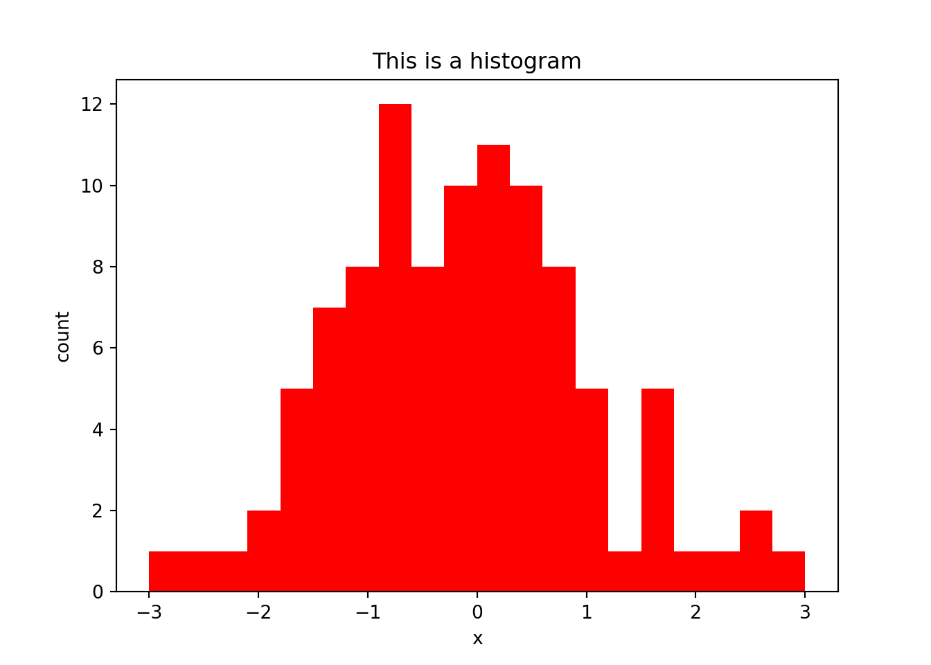
11.2 Quantile-Quantile Plots
After looking at the histogram, we may think that our data follows some specific distribution (e.g. normal distribution). Quantile-quantile plots can be used to see if two data sets are drawn from the same distribution. To do this, it plots the quantiles of each data set against one another. That is, it plots the 0th percentile of data set A (the minimum value) against the 0th percentile of data set B, the 50th percentiles (the medians) against each other, the 100th percentiles (the maximum values) against each other, etc. Simply, it sorts both data sets, and makes them both the same length by estimating any missing values, then plots a scatterplot of the sorted data. If the two data sets are drawn from the same distribution, this plot should follow the \(x = y\) identity line at all but the most extreme point.
We can use the api module from statsmodels to plot a QQ plot to see if our randomly generated array was indeed drawn from a normal distribution, by comparing x with a standard normal distribution (scipy.stats.distributions.norm). A 45 degree line is added to show the theoretical identity between the two distributions. The closer the points lie to this line, the closer the two distributions are:
import statsmodels.api as sm
sm.qqplot(x, line = '45', dist = scipy.stats.distributions.norm)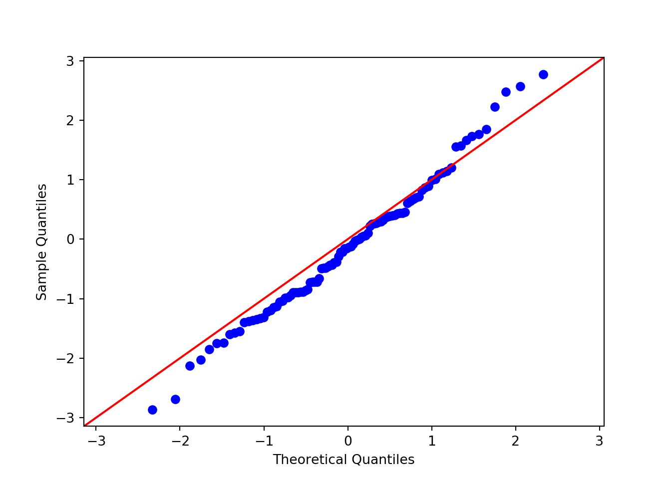
Indeed, these data seem to approximate a normal distribution.
11.3 Pie Chart
Now let’s say that we have a data set that shows the number of called peaks from a ChIPseq data set that fall into distinct genomic features (exons, introns, promoters and intergenic regions). One way to look at how the peaks fall would be to look at a pie graph, which shows proportions in a data set represented by slices of a circle:
peaknums  = [1400,900,200,150]
peaknames = ["exons", "intron", "promoter", "intergenic"]
p = plt.pie(peaknums, labels = peaknames)
plt.show()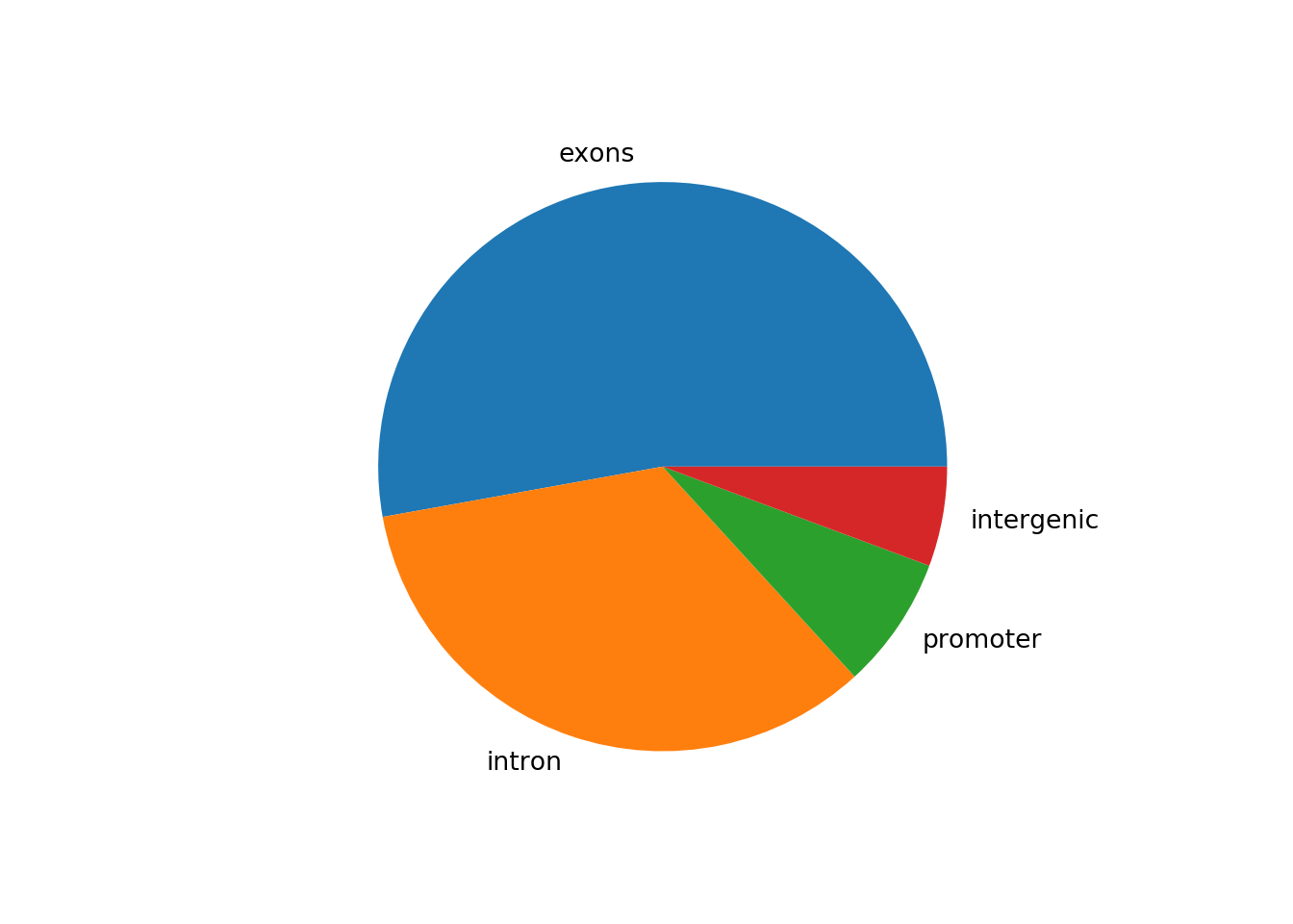
This figure shows that the majority of the peaks fall into exons.
11.4 Bar Plot
However, pie charts are typically discouraged by statisticians, because your eyes can often misjudge estimates of the area taken up by each feature. A better way of looking at data such as this would be in the form of a barplot:
b = plt.bar(peaknames, peaknums)
plt.show()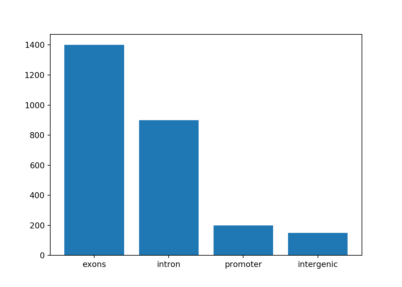
11.5 Line Plots
The pyplot function plot() is the standard plotting method for 2-dimensional data, and is used to plot paired data x and y against one another, using markers and/or lines. Plots such as these are useful for looking at correlation between two data sets. By default, the plot() function will plot a line plot:
plt.plot(x,y)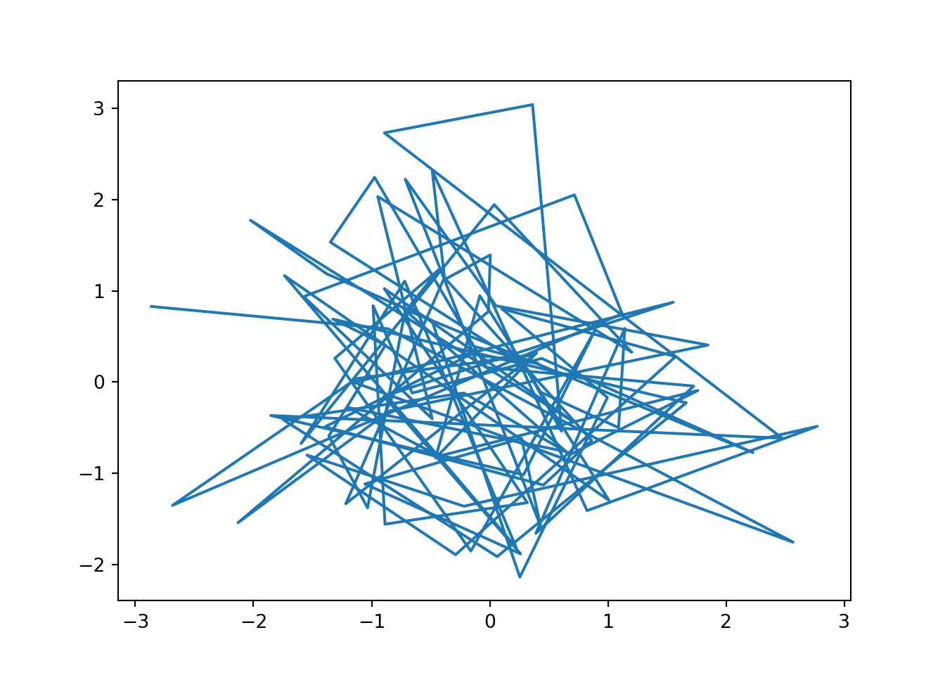
Note that this looks very messy. This is due to the fact that the line starts with the first pair of values ($x_1$, $x_2$), then plots a line to the second pair of values ($x_1$, $x_2$), and so on. Since x and y are completely random, there is no order from lowest to highest for either, and so we end up with this messy image. For a line plot, we need to sort the data so that the x-axis data run from left to right. Since both data sets need to remain paired, we only sort one data set, and use this ordering to rearrange both data sets using the argsort() method:
plt.plot(x[x.argsort()],y[x.argsort()])
plt.show()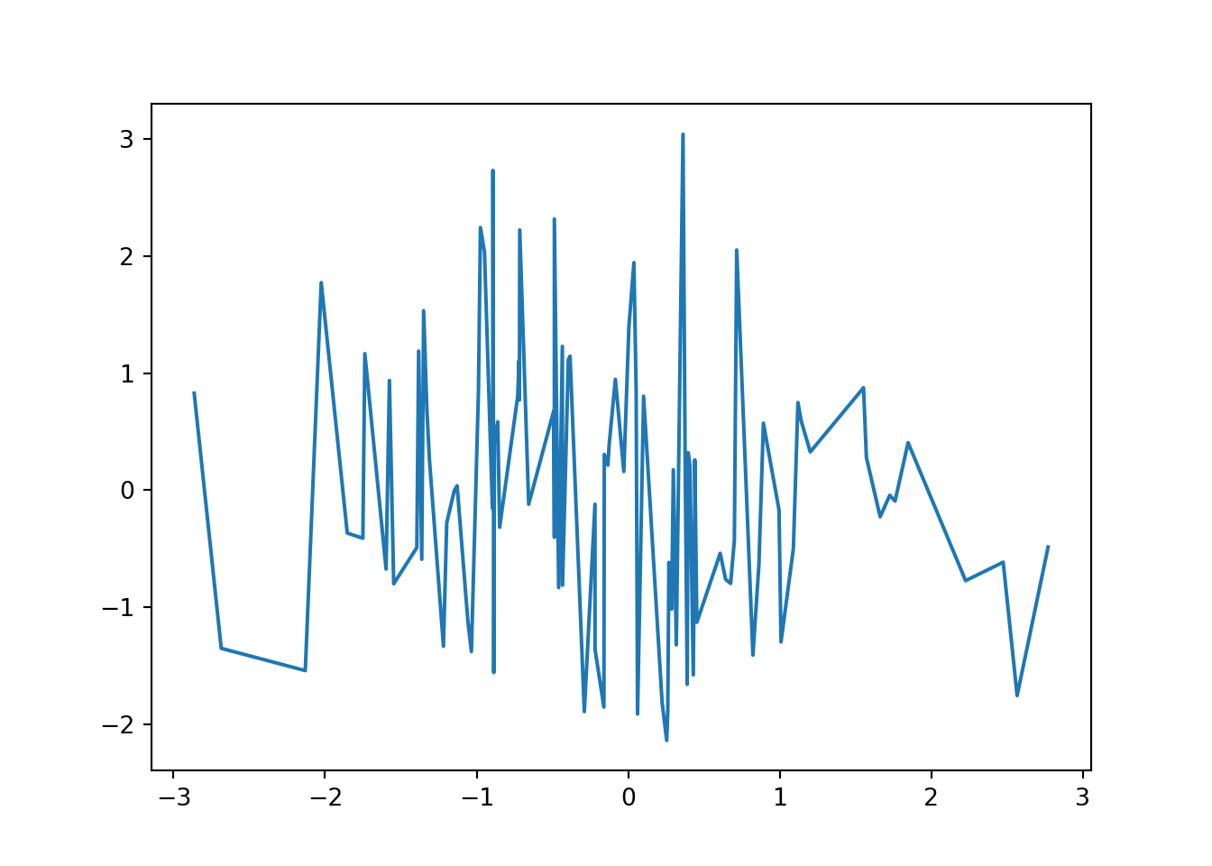
We can use a number of the arguments described above to modify this plot, including adding axis labels, a title, and some markers for each of the points:
plt.plot(x[x.argsort()],y[x.argsort()], marker = 'o', color = 'red', linestyle = '--')
plt.title("This is y vs. x")
plt.xlabel("This is x")
plt.ylabel("This is y")
plt.show()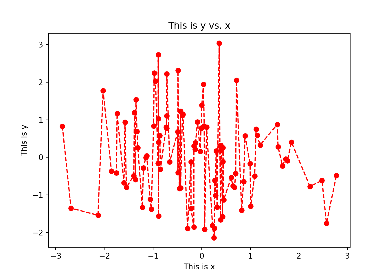
11.6 Scatterplots
Sometimes we may only want to look at the markers and not plot a line between them, for instance to save us worrying about ordering as we had to do above. This allows us to take a general look over the relationship between two numeric data sets. For instance, for every student in a class, we may have scores from tests taken at the start and at the end of the year, and we want to compare them against one another to see how they compare. We can use the same function, and simply set the linestyle to '':
plt.plot(x,y, color = "red", marker = 'o', markersize = 10, linestyle = '')
plt.title("This is y vs. x")
plt.xlabel("This is x")
plt.ylabel("This is y")
plt.show()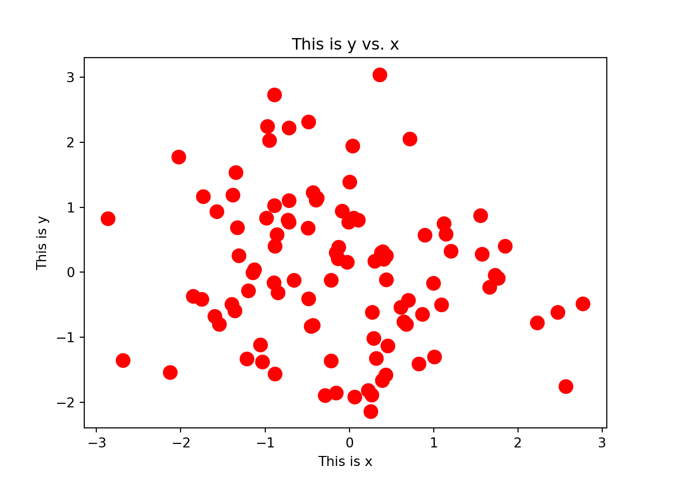
Here we have coloured all of our points a single colour by using the color = "red" argument. However, we may want to assign colours to each point separately by supplying an array of colours that is the same length as x and y. This means that we can set colours based on the data themselves, e.g. to colour male and female samples differently to one another, or to color points that exceed some threshold of interest. To do this, we can use the scatter() function, which can take a list of colors using the c argument:
## Create an array containing "black" for every element in x
mycols = np.repeat("black", len(x))

## Change the color based on the values in x and y
mycols[(x >  0.5) & (y >  0.5)] = "red"
mycols[(x < -0.5) & (y < -0.5)] = "blue"

## Plot the scatter plot
plt.scatter(x, y, color = mycols, marker = 'o')
plt.title("This is y vs. x")
plt.xlabel("This is x")
plt.ylabel("This is y")
plt.show()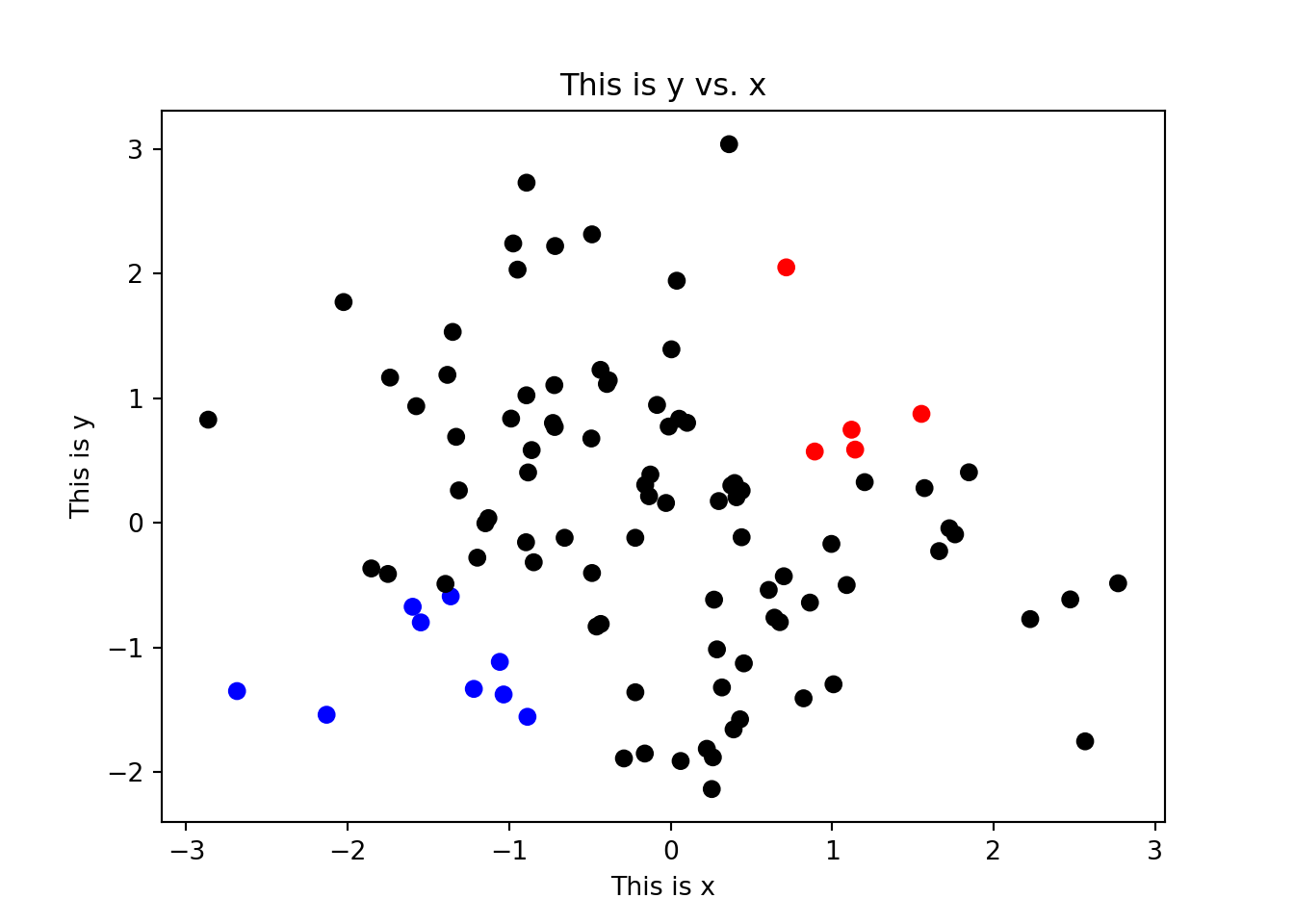
11.7 Boxplots
To compare the distribution of multiple numeric data sets, we can use boxplots. A boxplot shows the overal distribution by plotting a box bounded by the first and third quartiles, with the median highlighted. This shows where the majority of the data lie. Additional values are plotted as whiskers coming out from the main box. Multiple boxes can be plotted next to one another allowing you to compare similarlities or differences between them. This can be used for instance to compare distributions of two different data sets, or to compare a numeric value in a data set after separating out multiple classes (e.g. comparing different age groups). The plot produces a dict object:
bp = plt.boxplot([x,y])
plt.show()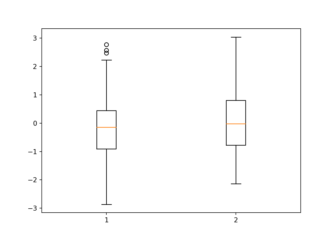
There are a number of arguments that can be supplied, including labels which allows you to specify the labels on the x-axis, notch which will add a notch into the boxplot to represent the confident interval, whis to determine the extent of the whiskers (any values not included within the whiskers are plotted as outliers), and widths to change the widths of the boxes:
bp = plt.boxplot([x,y], labels = ['x', 'y'], notch = 1, whis = 1, widths = [0.1, 1])
plt.show()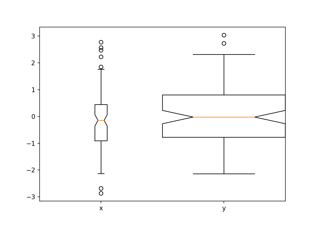
Pandas also has a boxplot() function which can take the data in the form of a DataFrame, which is useful for instance if you want to compare the distribution of expression values over all genes for a number of different samples. It will do a pretty good job of pulling out only the numeric columns by default, or you can specify which columns you would like to plot:
df = pd.DataFrame({'Name':['John', 'Paul', 'Jean', 'Paula'], 'Age':[37,33,40,35], 'Score':[99.3,92.6,97.5,92.6], 'Gender':['Male', 'Male', 'Female', 'Female']})
df.boxplot(column = ['Age', 'Score'])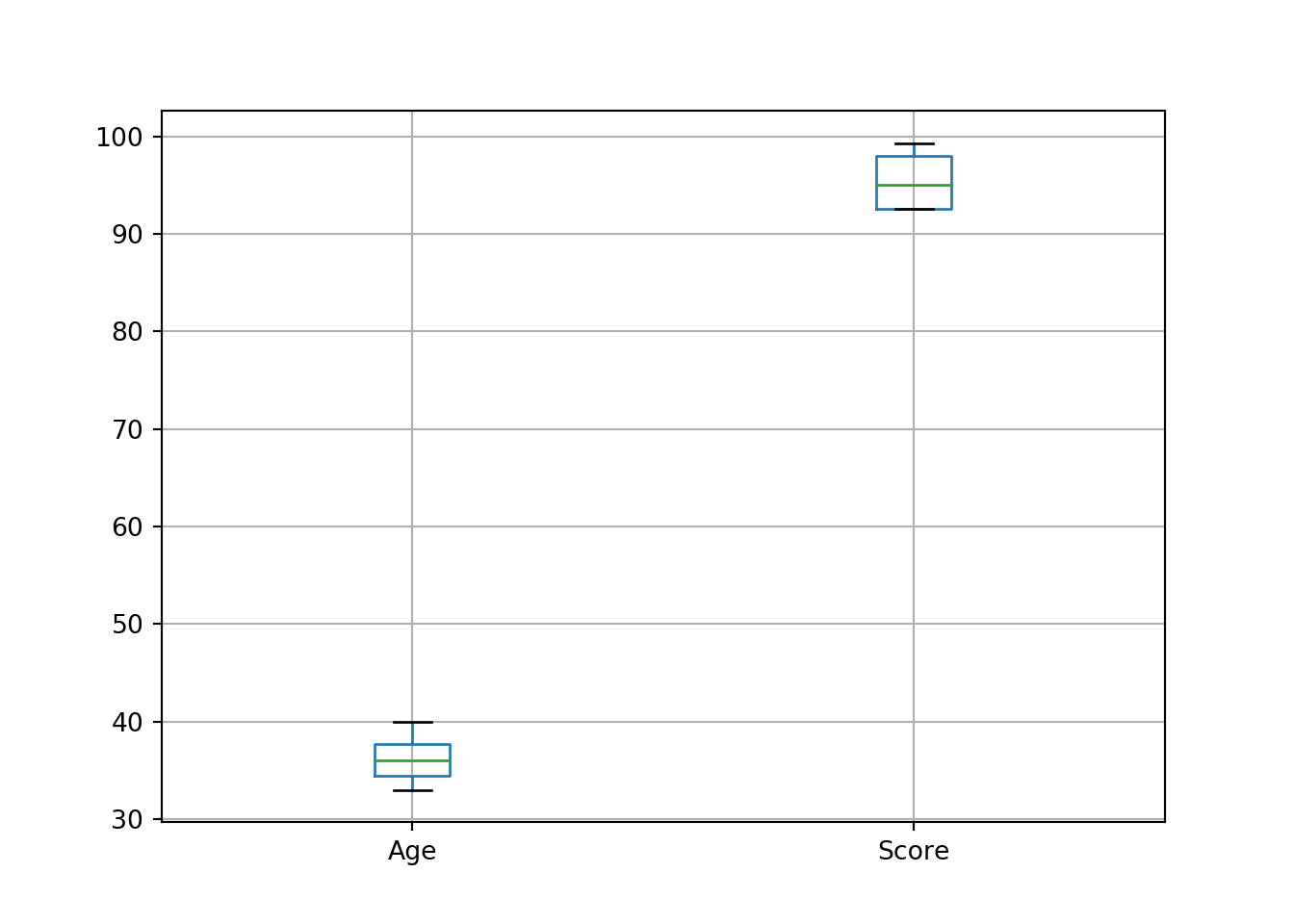
11.8 Seaborn package
The Seaborn package is an incredibly powerful package for plotting using DataFrames, and is quite similar to the `ggplots2 package in R. It makes defining the components of a plot much simpler in cases when data are stored correctly in DataFrame objects. It is beyond the scope of this tutorial to go into this in too much detail, but the idea is to use the names of the variables in the DataFrame to define various elements of the plot. For instance, in the following plot, we split data on the x-axis by their Gender, and then for each subset we plot the score:
import seaborn as sb
sb.boxplot(x = 'Gender', y = 'Score', data = df)
Seaborn will use some defaults to make this figure look nice, such as filling in the boxes automatically, labelling the axes, etc. However, a lot of additional parameters can be set to change these. If you are interested, I recommend spending some time looking over this package to see the number of options available to you.
11.9 Subplots
By default, the graphics device will plot a single figure only. The subplots() function can be used to create multiple subplots within a single plot. By default, the method will create a single figure and a single axis, but by including the number of rows and columns the axis can contain a list of multiple axes for plotting. Each element of the list can then be used to build up the plot as described above:
fig, subplt = plt.subplots(2, 1)
subplt[0].plot(x,y)
subplt[1].plot(x,-y)
To plot them side-by side instead, this is as simple as changing the arguments to subplots():
fig, subplt = plt.subplots(1,2)
subplt[0].plot(x,y)
subplt[1].plot(x,-y)
For multiple rows and columns, the axis output is a 2-dimensional NumPy array so each plot can be accessed and modified using square brackets notation:
fig, subplt = plt.subplots(2,2)
subplt[0,0].plot(x,y)
subplt[0,0].set_title("Plot1")
subplt[0,1].plot(x,-y)
subplt[0,1].set_title("Plot2")
subplt[1,0].plot(-x,y)
subplt[1,0].set_title("Plot3")
subplt[1,1].plot(-x,-y)
subplt[1,1].set_title("Plot4")
You can also create specific objects for each of the plots directly when calling subplots():
fig, ((plt1,plt2), (plt3,plt4)) = plt.subplots(2,2)
plt1.plot(x,y, color = "red")
plt1.set_title("Plot1")
plt2.plot(x,-y, color = "blue")
plt2.set_title("Plot2")
plt3.plot(-x,y, color = "orange")
plt3.set_title("Plot3")
plt4.plot(-x,-y, color = "green")
plt4.set_title("Plot4")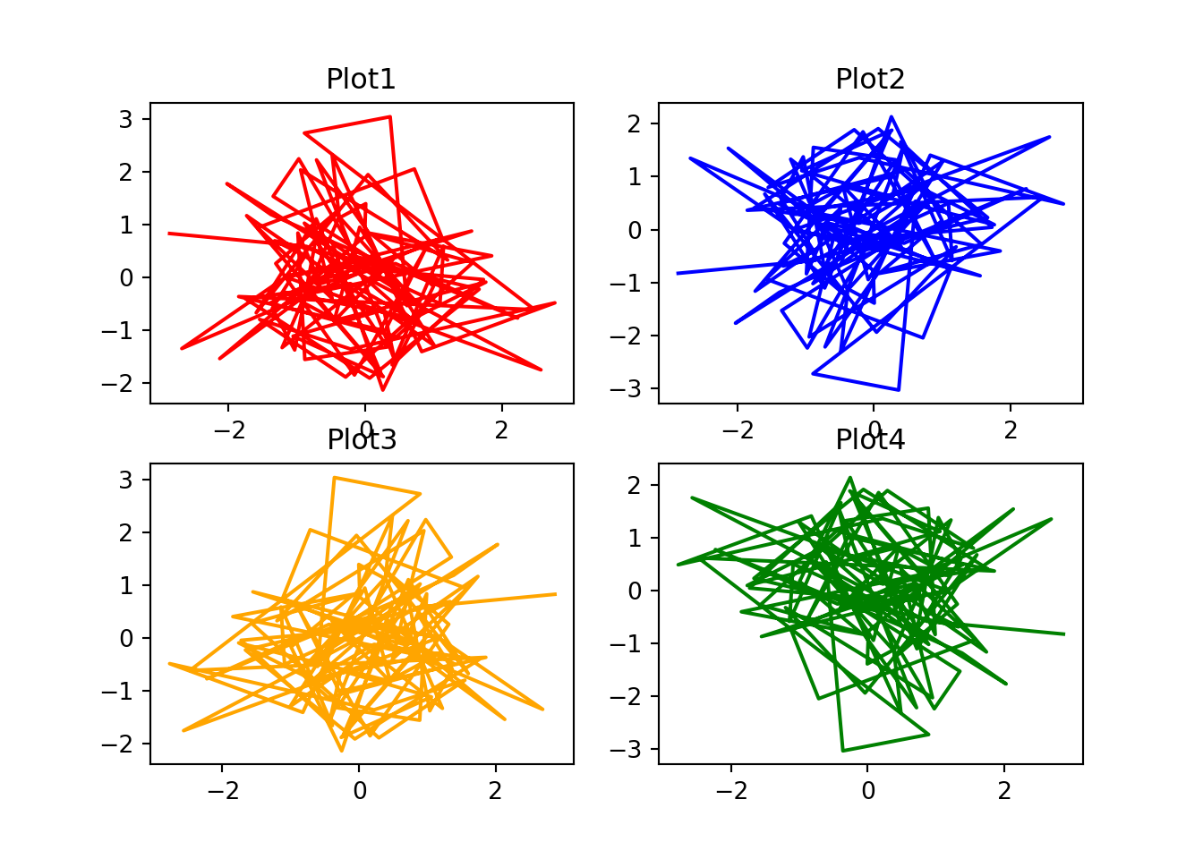
By default, each plot will have its axis limits calculated independently, but it is possible to use the sharex and sharey arguments to share the axis limits across all plots:
fig, ((plt1,plt2), (plt3,plt4)) = plt.subplots(2,2, sharex = True, sharey = True)
plt1.plot(x,2*y, color = "red")
plt1.set_title("Plot1")
plt2.plot(x,-y, color = "blue")
plt2.set_title("Plot2")
plt3.plot(-3*x,2*y, color = "orange")
plt3.set_title("Plot3")
plt4.plot(-x,-4*y, color = "green")
plt4.set_title("Plot4")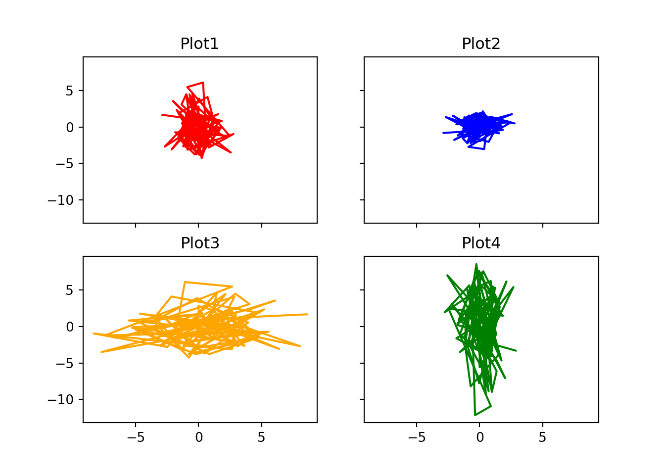
11.10 Saving Figures
By default, figures are generated in a separate window by using the show() function. However, you can save the figure to an external file by using the savefig() function. The output format can be defined simply by adding a suffix to the file – .jpg, .pdf, .png, etc.:
plt.plot(x,y)
plt.savefig("test.png")
To change the size of the image, you can specify the size of the figure (in inches) before generating the plot using the figsize argument in the figure() method. To define the resolution of the output figure, you can set the dpi argument for savefig() to change the dots per inch value. Also, by default the margins for output figures can be quite large, so you can use the `bbox_inches’ argument to change this:
plt.figure(figsize=(10,10))
plt.plot(x,y)
plt.savefig("test.png", bbox_inches='tight')
12 Example Analysis
12.1 Introduction
This is just a simple example analysis to give you an idea of the sort of things that we can do with Python. Suppose that we have two experiments, each looking at the effects on gene expression of using a particular drug (“Drug A” and “Drug B”). For each experiment we have two samples; one showing the gene expression when treated with the drug, and the other showing the gene expression when treated with some control agent. Obviously in a real experiment, we would have many replicates, but here we have \(n=1\). We want to do the following:
- For each drug, we want to get the fold change for each gene
- For each drug, we want to identify the genes that are significantly changed when using the drug
- We want to compare the results for Drug A with those from Drug B to find genes that are affected similarly by both drugs
- We want to plot the correlation between the fold change values for the two drugs to see how similar they are
For this, we will need four files. These files are in a tab-delimited text format. They are tables of values where each row is separated by a new line, and each column is separated by a tab character (\t). These files can be created by and read into Excel for ease of use. To avoid errors when reading in files from text, it is good practice to ensure that there are no missing cells in your data. Instead try to get into the habit of using some “missing”" character (e.g. NA).
| File Name | Description |
|---|---|
| experiment1_control.txt | Expression levels for ctrl in expt 1 |
| experiment1_drug.txt | Expression levels for drug A in expt 1 |
| experiment2_control.txt | Expression levels for control in expt 2 |
| experiment2_drug.txt | Expression levels for drug A in expt 2 |
12.2 Load Data
First let’s load in the data:
expt1_ctrl = pd.read_csv("experiment1_control.txt", sep = "\t")
expt1_drug = pd.read_csv("experiment1_drug.txt",    sep = "\t")
expt2_ctrl = pd.read_csv("experiment2_control.txt", sep = "\t")
expt2_drug = pd.read_csv("experiment2_drug.txt",    sep = "\t")
Each of these files contains two columns; the gene name and some value that represents the expression level for that gene (assume that these values have been calculated after pre-processing, normalisation, etc.).
In all of these cases, the list of gene names is identical, and in the same order which means that we could compare row 1 from the control-treated file with row 2 from the drug-treated file to get all of the comparisons. However, in a real data set you will not know for sure that the gene names match so I recommend merging the files together into a single data frame to ensure that all analyses are conducted on a gene by gene basis on the correct values.
We therefore create a single DataFrame for both experiments using the merge() command:
expt1 = pd.merge(expt1_ctrl, expt1_drug, on = "GeneName", suffixes = ("_Control", "_Drug"))
expt2 = pd.merge(expt2_ctrl, expt2_drug, on = "GeneName", suffixes = ("_Control", "_Drug"))
expt1.head()
## GeneName Expression_Control Expression_Drug
## 0 gene1 64 48
## 1 gene2 50 62
## 2 gene3 74 73
## 3 gene4 31 34
## 4 gene5 63 66expt2.head()## GeneName Expression_Control Expression_Drug
## 0 gene1 55 60
## 1 gene2 51 51
## 2 gene3 77 74
## 3 gene4 23 22
## 4 gene5 72 10112.3 Calculate Fold Change
Now we calculate the fold change for each gene by dividing the drug-treated expression by the control expression. To avoid divide by zero errors, we can set a minimum expression value. This will also ensure that we are only looking at expression changes between significant expression values. Since we want to do the same thing to both the experiment 1 and the experiment 2 data sets, it makes sense to write a single function to use for both. We will use the apply() function from Pandas to calculate over every row in the DataFrame:
def get_fold_change(x, min_expression = 10):
  ctrl_val = x["Expression_Control"]
  drug_val = x["Expression_Drug"]
  if ctrl_val < min_expression:
    ctrl_val = min_expression
  if drug_val < min_expression:
    drug_val = min_expression
  return drug_val/ctrl_val
expt1['FoldChange'] = expt1.apply(get_fold_change, axis = 1)
expt2['FoldChange'] = expt2.apply(get_fold_change, axis = 1)
12.4 Compare Data
Now let’s find the genes that are upregulated and downregulated in each experiment. Due to the lack of replicates, we do not have any estimate for the variance of these genes, so we cannot use any hypothesis testing methods such as a t-test. Instead, we will have to make do with using a threshold on the fold change:
fold_change_threshold = 1.5
expt1_up   = expt1[expt1['FoldChange'] >= fold_change_threshold]['GeneName']
expt1_down = expt1[expt1['FoldChange'] <= 1/fold_change_threshold]['GeneName']
expt2_up   = expt2[expt2['FoldChange'] >= fold_change_threshold]['GeneName']
expt2_down = expt2[expt2['FoldChange'] >= 1/fold_change_threshold]['GeneName']
So let’s see which genes are changing:
print("Upregulated in Experiment 1:", expt1_up.str.cat(sep = ", "))## Upregulated in Experiment 1: gene8, gene12print("Downregulated in Experiment 1:", expt1_down.str.cat(sep = ", "))## Downregulated in Experiment 1: gene32, gene46print("Upregulated in Experiment 2:", expt2_up.str.cat(sep = ", "))## Upregulated in Experiment 2: gene8, gene18, gene50print("Downregulated in Experiment 2:", expt2_down.str.cat(sep = ", "))## Downregulated in Experiment 2: gene1, gene2, gene3, gene4, gene5, gene6, gene7, gene8, gene9, gene10, gene11, gene12, gene13, gene14, gene15, gene16, gene17, gene18, gene19, gene20, gene21, gene23, gene24, gene25, gene26, gene27, gene28, gene29, gene30, gene31, gene32, gene33, gene34, gene35, gene36, gene37, gene38, gene39, gene40, gene41, gene42, gene44, gene45, gene46, gene47, gene48, gene49, gene50So we now have the genes that change when each of the drugs is used. But now we want to compare the two drugs together. First, let’s see if there are any genes similarly affected by both drugs. We can do this using the intersect1d() function from NumPy which gives the intersect of two arrays:
common_up   = pd.Series(np.intersect1d(expt1_up, expt2_up))
common_down = pd.Series(np.intersect1d(expt1_down, expt2_down))
print("Upregulated in Experiment 1 and Experiment 2:",   common_up.str.cat(sep = ", "))
## Upregulated in Experiment 1 and Experiment 2: gene8print("Downregulated in Experiment 1 and Experiment 2:", common_down.str.cat(sep = ", "))## Downregulated in Experiment 1 and Experiment 2: gene32, gene46So we can see that only one gene is similarly affected by both drugs (“gene8”). Now let’s plot a figure to see how the fold change differs between the two drugs:
fc = pd.merge(expt1[['GeneName', 'FoldChange']], expt2[['GeneName', 'FoldChange']], on = "GeneName", suffixes = ["_Experiment1", "_Experiment2"])
plt.scatter(np.log2(fc["FoldChange_Experiment1"]),
            np.log2(fc['FoldChange_Experiment2']),
            marker = "o", color = "red")
plt.xlim(-2,2)
## (-2, 2)plt.ylim(-2,2)## (-2, 2)plt.title("Experiment1 vs Experiment2")
plt.xlabel("log2(Experiment1 Fold Change)")
plt.ylabel("log2(Experiment2 Fold Change)")
plt.show()
This figure shows that the effect on the gene expression is actually quite different for the two drugs. We can also see this by looking at the correlation between the two experiments:
scipy.stats.pearsonr(fc["FoldChange_Experiment1"], fc["FoldChange_Experiment2"])## (0.0838161376824968, 0.5627922240659949)We can therefore conclude that the effect of the drug on gene expression is quite different between the two experiments.
Sam Robson
Lead Bioinformatician at the Centre for Enzyme Innovation
Lead Bioinformatician at the Centre for Enzyme Innovation