6.1 Delayed uploads

One of the criticisms that comes up regarding Mimi’s practice is that it sometimes takes a long time for the data to be uploaded to Strava. I believe that it is typically up within a couple of hours (EDIT - there were also times when the uploads were not made for several days which is obviously more than a delay in tranferring the data), but many people suggest that anything longer than 15 minutes is unacceptable as it provides time to doctor the data. I mean, I guess that this is true, but it is my understanding that, given Mimi’s lack of technological prowess, her crew is using the method that requires the least amount of knowledge; that being syncing to a phone via Bluetooth, which will then upload to Movescount when there is a wifi or mobile data signal. I do this sometimes with my own runs and it takes bloody ages to sync, and that doesn’t take into account the time to then takes to upload it from the phone to Movescount, dealing with blackspots, etc. So it does not surprise me in the least that she rarely uploads things within 15 minutes of stopping. This is not evidence based by any means, just an observation from my own experience (and something others have pointed out). Is this good practice for somebody out to claim a world record? Perhaps not. Is it evidence of subterfuge? I don’t know, but personally I doubt it.

6.2 “Mimi is pausing her watch”

In page 201 of the LetsRun thread, user So Far Today says the following:

Elapsed time is total time from start of the day until end of the day. Sandy’s Strava is based on total elapsed time. Mimi’s excludes lunch breaks, and it appears it it also excludes other mini-breaks. If you want to figure out actual running time for Sandy remove the lunch breaks from the total elapsed time.

Now, these guys have been looking into this in a heck of a lot more detail than I have, so I apologise if I have got this wrong here or misunderstood. But the idea that Mimi’s data excludes mini-breaks disagrees with something that I noticed right at the start of this analysis. Let’s look at the time difference between successive data points for Mimi’s data using the table() function which will simply count the number of occurrences of each time delay between data points:

lapply(all_gpx[["MimiAnderson"]], FUN = function (x) table(x[["time.diff"]]))

$MimiAnderson_170828_preUSA

0 1 2 5 1 4160 4 1

$MimiAnderson_171001_afternoon

0     1     2 
1 25883    11 

$MimiAnderson_171002_afternoon

0     1     2 
1 26174    31 

$MimiAnderson_171002_morning

0     1     2     3 
1 29046    44     1 

$MimiAnderson_171003_afternoon

0     1     2 
1 10926    12 

$MimiAnderson_171003_morning

0     1     2     3 
1 30896     7     1 

$MimiAnderson_171004_afternoon

0     1     2     3     4 
1 24567    19     1     1 

$MimiAnderson_171004_morning

0     1     2 
1 28343     6 

$MimiAnderson_171005_afternoon

0     1     2 
1 18492    42 

$MimiAnderson_171005_morning

0     1     2     3 
1 32400    34     2 

$MimiAnderson_171006_afternoon

0     1     2     3 
1 26461     7     1 

$MimiAnderson_171006_morning

0     1     2     7 
1 27747    42     1 

$MimiAnderson_171007_afternoon

0     1     2     3 
1 21215    36     1 

$MimiAnderson_171007_morning

0     1     2 
1 32114    27 

$MimiAnderson_171012_morning

0     1     2 
1 28411    17 

So every run has one 0 (which is a result of the way that I have calculated the time difference, so the first value is always 0), a few sporadic 2-7 sec intervals (presumably due to brief signal drop out and the like), but the vast majority are 1 sec. This is because Mimi has her watch set to 1 sec recording, and leaves it on for the duration of the run. From this I suggest that the assertion made that Mimi stops her watch for lunch breaks etc. is false.

My watch is set to the same sampling rate, and I see exactly the same thing with my data (albeit with fewer errant digits):

lapply(all_gpx[["Mine"]], FUN = function (x) table(x[["time.diff"]]))

$mine_170514

0 1 2 1 9790 1

$mine_170521

0 1 2 1 6860 1

$mine_170525

0 1 1 3056

$mine_170603

0 1 1 5531

$mine_170618

0     1 
1 11297 

Interestingly, however, when we look at Sandra’s data we see a completely different result:

lapply(all_gpx[["SandraVi"]], FUN = function (x) table(x[["time.diff"]]))

$SandraVi_171002

0 1 2 3 4 5 6 7 8 9 10 11 12 13 14 15 16 17 1 82 79 77 61 57 48 51 65 126 332 348 335 160 51 14 4 1 18 21 22 29 30 32 35 38 39 43 47 48 51 54 55 61 63 66 1 1 2 1 1 1 1 1 3 1 1 1 2 1 1 1 1 1 86 89 133 1 1 1

$SandraVi_171003

0 1 2 3 4 5 6 7 8 9 10 11 12 13 14 1 243 238 233 187 192 172 210 305 1459 1424 401 142 54 40 15 16 17 18 19 20 21 22 23 24 25 27 28 30 31 17 7 1 2 4 1 4 2 1 2 2 1 1 1 1 33 34 35 36 37 39 40 41 44 45 46 47 49 50 51 2 1 1 1 1 1 2 1 1 1 1 1 1 1 1 52 53 55 57 58 59 60 63 64 65 66 73 79 82 83 2 3 3 1 1 1 1 1 1 1 1 1 1 1 1 88 89 97 100 102 113 118 119 133 136 162 166 168 183 223 1 1 1 1 1 1 1 1 1 1 1 1 1 1 1 249 266 1 1

$SandraVi_171004

0 1 2 3 4 5 6 7 8 9 10 11 12 13 14 1 299 425 356 333 267 311 311 697 1708 1022 327 157 76 33 15 16 17 18 19 20 21 22 23 24 26 27 28 29 32 26 15 6 6 1 1 1 3 1 3 1 1 3 1 1 33 35 36 37 39 41 43 44 49 50 51 52 55 56 57 2 2 1 1 4 1 1 1 1 1 2 1 1 2 1 58 59 61 62 64 67 70 74 75 84 88 94 98 130 149 1 1 2 1 1 2 1 1 1 1 1 3 1 1 1 169 1

$SandraVi_171005

0 1 2 3 4 5 6 7 8 9 10 11 12 13 14 1 173 167 157 133 156 129 158 400 1891 1393 259 109 53 55 15 16 17 18 19 20 21 22 23 24 26 27 29 30 32 16 6 5 2 1 5 1 1 2 1 1 1 1 1 1 33 34 35 36 37 39 41 44 46 49 50 52 61 68 74 2 1 1 1 2 1 1 1 1 1 3 1 1 2 1 75 76 93 128 138 140 145 153 163 233 1 1 1 1 2 1 1 2 2 1

$SandraVi_171006

0 1 2 3 4 5 6 7 8 9 10 11 12 13 14 1 112 128 123 132 115 122 101 291 1658 1696 358 85 42 33 15 16 17 18 19 20 24 27 28 32 35 37 42 46 49 8 5 4 2 1 2 1 2 1 2 1 1 1 1 2 51 57 58 60 65 67 76 77 78 86 88 90 96 98 99 1 1 1 1 1 1 1 1 1 1 2 1 1 1 1 106 108 109 126 128 129 147 164 173 196 205 1 1 1 1 1 1 1 1 1 1 1

$SandraVi_171007

0 1 2 3 4 5 6 7 8 9 10 11 12 13 14 1 57 85 83 73 81 74 64 197 2038 1707 275 95 64 39 15 16 17 18 22 23 27 28 31 32 38 39 40 42 45 17 11 2 1 2 1 1 5 2 1 1 1 3 3 1 46 49 53 54 55 60 65 67 77 84 109 115 126 128 149 2 1 1 2 1 1 1 1 1 1 1 1 1 1 1 151 154 157 181 182 189 225 1 1 1 1 1 1 1

There is no one time difference that stands out as the most common. Instead, the time differences between her data points span a large range, with the majority being about 8-11 secs apart. I suspect that this means that Sandra’s watch is set to sample every 10 seconds or so. In addition, there are a lot more longer pauses seen, sometimes up to 4 minutes. Whether this is a result of random fluctuations due to the higher sampling rate, or is the result of pausing the watch at certain times, I do not know. I am most definitely not suggesting there is anything wrong with this, I just think that the better approach is to leave it running the whole time, and it is Mimi who is doing this and not Sandra.

Note also that this means that Sandra’s data therefore has an order of magnitude fewer data points than Mimi’s does, since Mimi’s data is less smoothed out. This can be seen if we calculate the number of data points for each run and then show the distribution for Mimi and Sandra separately (note that each of Mimi’s runs is actually only half of her distance for the day):

plot_dat <- list()
for (n in c("MimiAnderson", "SandraVi")) {
  plot_dat[[n]] <- data.frame(Name = n,
                              nPoints = sapply(all_gpx[[n]], FUN = nrow))
}
plot_dat <- do.call(rbind.data.frame, plot_dat)
ggplot(aes(x = nPoints, fill = Name), data = plot_dat) + 
  geom_density(alpha = 0.25)                           +
  ggtitle("Number of Data Points Per Run")             +
  xlab("Number of Data Points")                        + 
  ylab("Density")                                      +
  theme(axis.title = element_text(size = 10), 
        plot.title = element_text(size = 15, 
                                  face = "bold"))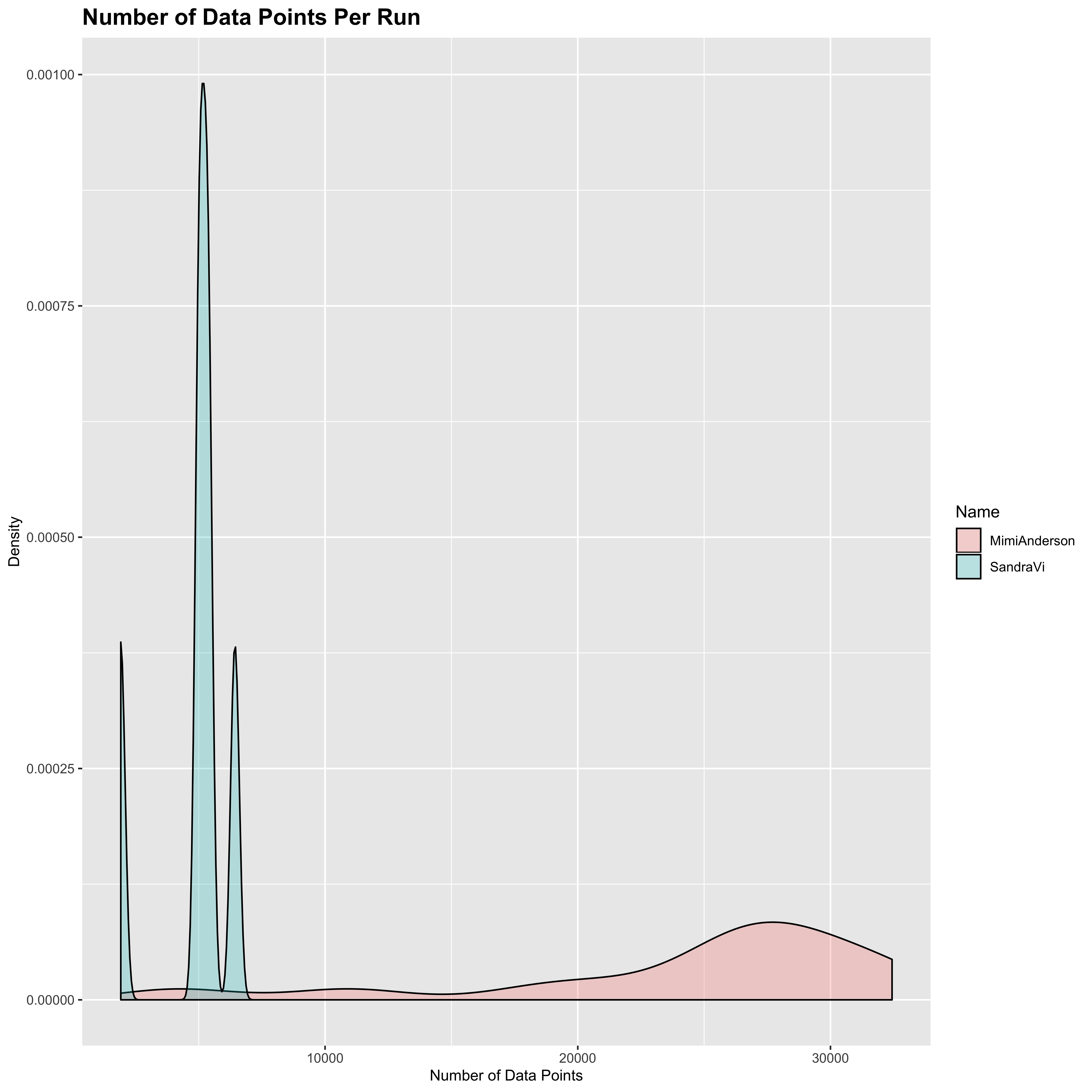

I’m not sure whether the people on LetsRun have been working on the assumption that both data sets were using the same parameters, but it is pretty clear to me that the sampling rate at least is different between the two runners. There may also be differences in the accuracy - perhaps the crews could confirm one way or another. Whilst the overall approach taken by Sandra is clearly the better of the two, the 1 sec sampling rate used by Mimi is the better option for the Strava data.

6.3 Dodgy fluctuations in cadence data

One issue that has been raised is the fact that in most of Mimi’s runs, we occasionally see severe fluctuations in the cadence, which spikes up above 200 at times. This is absolutely true, which can be seen when we plot the cadence values over time. The following function will plot the raw cadence values against the cumulative time (in secs) from the start of each run:

plot_cadence_over_time <- function (n, smooth = FALSE) {
  plot_dat <- list()
  for (r in names(all_gpx[[n]])) {
    if (smooth) { ## Smooths the data if requested - see below
      cad <- runmed(all_gpx[[n]][[r]][["extensions.cadence"]], 11)
    } else {
      cad <- all_gpx[[n]][[r]][["extensions.cadence"]]
    }
    plot_dat[[r]] <- data.frame(Run     = r,
                                Time    = cumsum(all_gpx[[n]][[r]][["time.diff"]]),
                                Cadence = cad)
  }
  plot_dat <- do.call(rbind.data.frame, plot_dat)
  ggplot(aes(x = Time, y = Cadence, color = Run), data = plot_dat) + 
    geom_point()                                                   + 
    facet_grid(Run ~ .)                                            + 
    ggtitle(paste(n, "Cadence Over Time"))                         + 
    xlab("Time (sec)")                                             + 
    ylab("Cadence (spm)")                                          +
    theme(axis.title = element_text(size = 10), 
          plot.title = element_text(size = 15, 
                                    face = "bold"))                + 
    ylim(0,500) # Limits the plot to a maximum of 500 which will exclude a small number of outliers for Mimi
}

Then we can look at Mimi’s raw cadence over time:

plot_cadence_over_time("MimiAnderson")
## Warning: Removed 120 rows containing missing values (geom_point).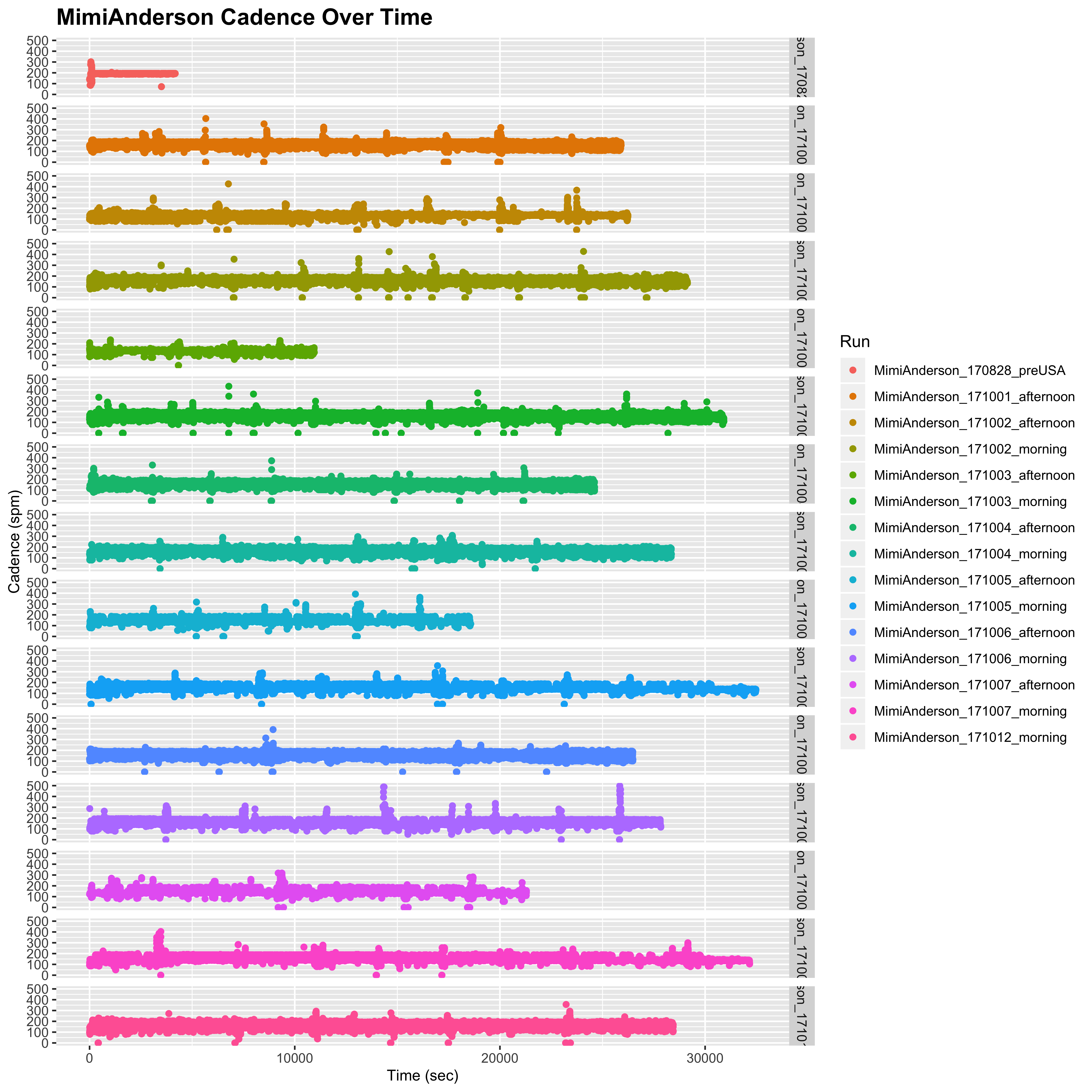

So there is no denying that these very high cadence values do exist in Mimi’s data. If, however, we look at Sandra’s data we do not see as many of these fluctuations. However, fluctuations are indeed still present, particularly for the shorter day on 2nd October, although they are nowhere near as high as those of Mimi (250 rather than 500):

plot_cadence_over_time("SandraVi")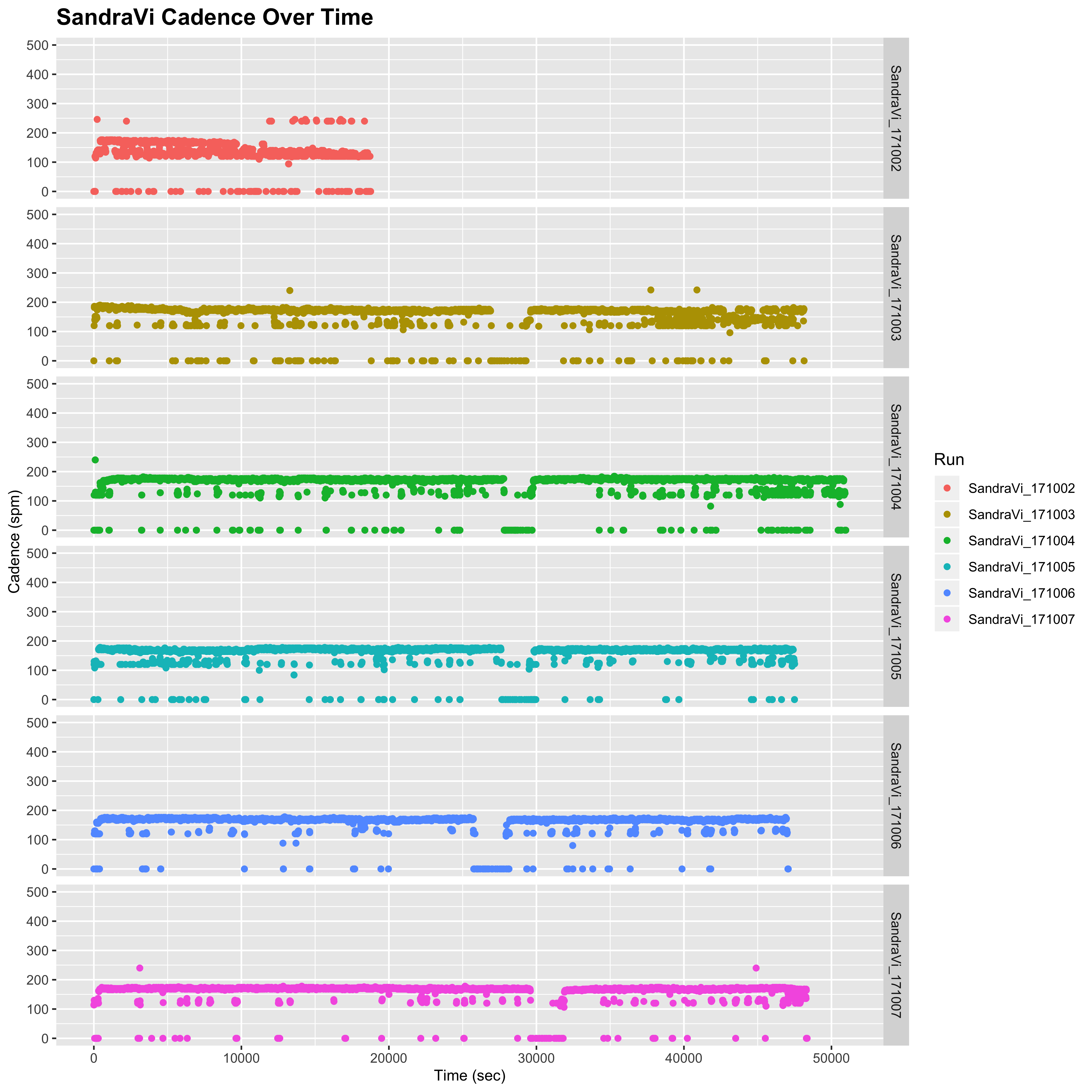

Note that here we can make out the lunch breaks in Sandra’s data, whereas Mimi has her runs split into morning and afternoon.

However, as discussed above, Mimi’s data is much deeper than Sandra’s. Sandra’s data has already undergone some smoothing, so it is likely that these blips are cancelled out by smoothing over a 10 second interval. Indeed, if we smooth Mimi’s data using a running median over an 11 sec window (which replaces the data points with a running average of the data point with the 5 data points either side) to approximate the 10 sec capture, we indeed see a much smoother distribution with these extreme values reduced to be more in keeping with what we see for Sandra.

plot_cadence_over_time("MimiAnderson", smooth = TRUE)
## Warning: Removed 85 rows containing missing values (geom_point).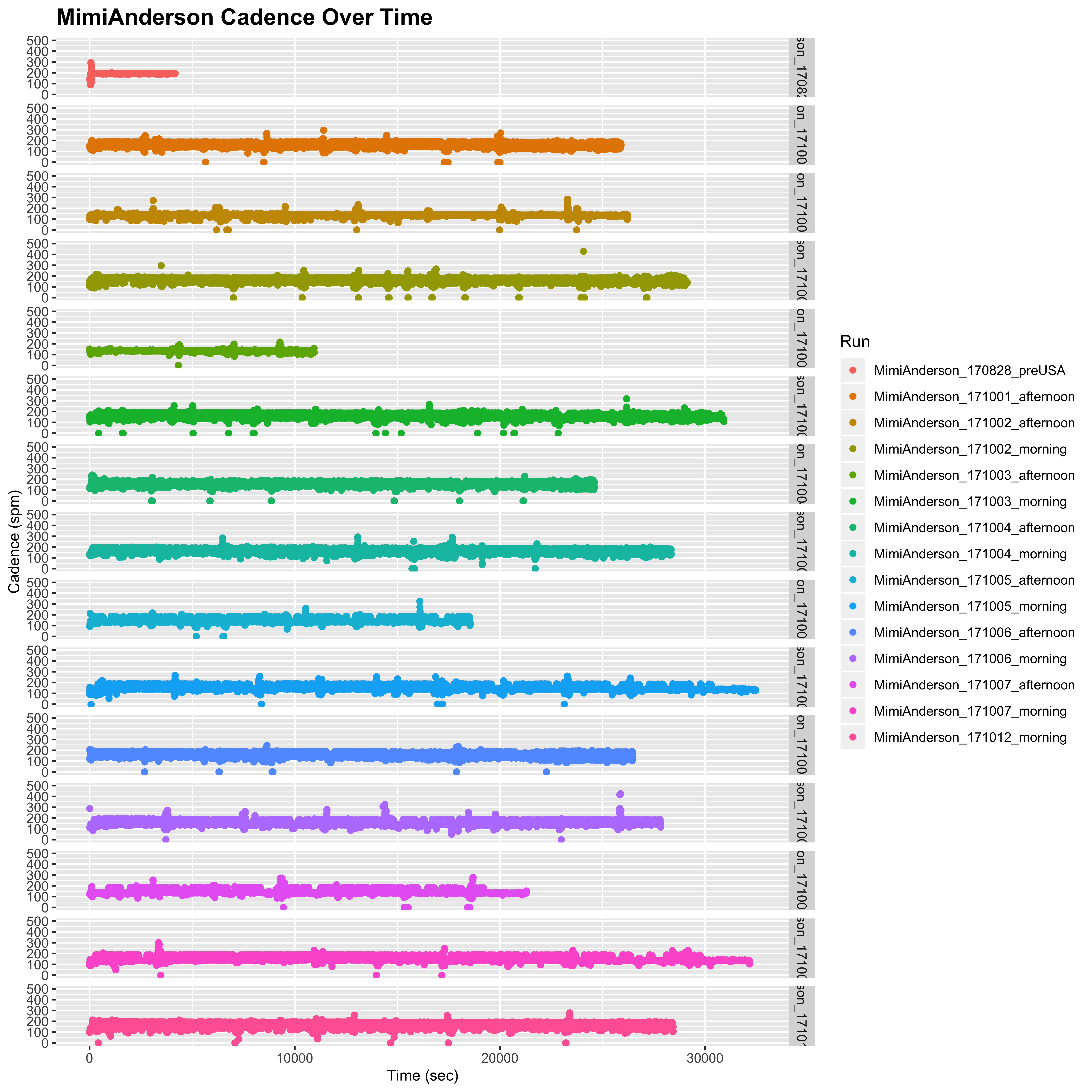

It would appear that these very high fluctuations are a result of the increased sampling rate, although I do note that I do not see these sorts of fluctuations in my own 1 sec capture data:

plot_cadence_over_time("Mine")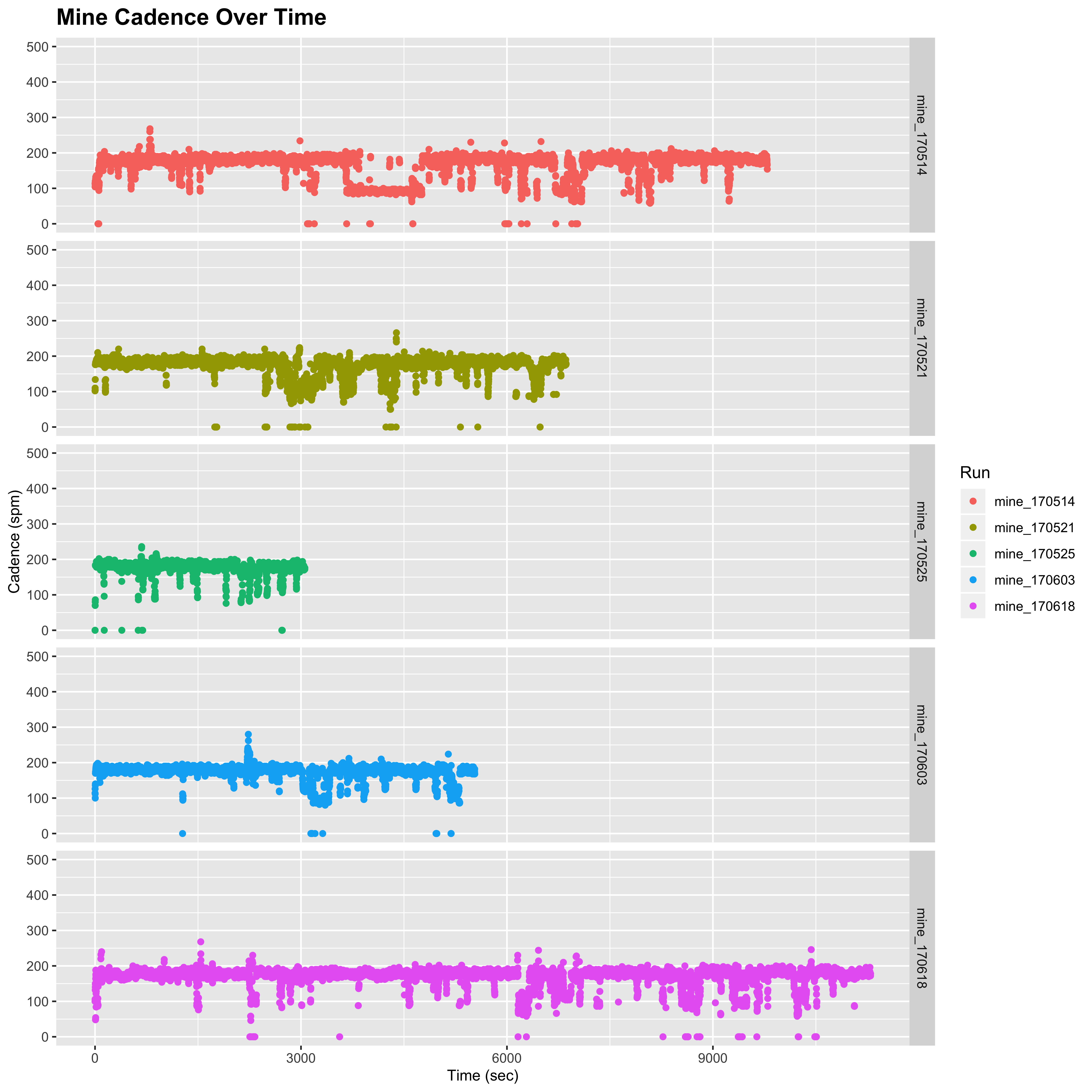

This may simply be due to the fact that I am not running through so many different areas, many of which may have different GPS signals that affect the capture. Another possibility is that the accuracy of our watches is set to different modes. Mine is set to “Best”, but I have no idea what Mimi’s is set to. One idea that I had was to ask her to set one of her watches to 10 sec capture and upload both in parallel at the end of one of her runs. However, unfortunately it seems that this is no more an option. I am going to hunt through to find some longer runs in my personal data to see if this crops up in any of my more remote jaunts, but for now I don’t have an answer.

6.4 Mimi running in the 185-195 steps per minute range:

Continuing with the cadence data, another issue that has cropped up several times is the fact that Mimi regularly runs in the 185-195 spm. Indeed, if we look at the distribution of the cadence in a histogram rather than looking at it over time, this certainly seems to be the case.

The following function will plot the above data as a series of overlaid density plots (note that I am smoothing the density estimates here slightly to make the overall distribution clearer and less spiky for the samples with fewer data points):

plot_cadence_density <- function (n) {
  plot_dat <- list()
  for (r in names(all_gpx[[n]])) {
    if (r == "MimiAnderson_170828_preUSA") next # Skip the pre-transcon run
    plot_dat[[r]] <- data.frame(Run     = r,
                                Cadence = all_gpx[[n]][[r]][["extensions.cadence"]])
  }
  plot_dat <- do.call(rbind.data.frame, plot_dat)
  vwalk    <- Mode(plot_dat[["Cadence"]][plot_dat[["Cadence"]] > 100 & plot_dat[["Cadence"]] < 150]) ## Walking
  vrun     <- Mode(plot_dat[["Cadence"]][plot_dat[["Cadence"]] > 150 & plot_dat[["Cadence"]] < 200]) ## Running
  ggplot(aes(x = Cadence, color = Run), data = plot_dat) + 
    geom_density(alpha = 0.25, adjust = 3)               + 
    xlim(0,300)                                          + 
    ggtitle(paste(n, "Cadence Distribution"))            + 
    xlab("Cadence (spm)")                                + 
    ylab ("Density")                                     +
    theme(axis.title = element_text(size = 10), 
          plot.title = element_text(size = 15, 
                                    face = "bold"))      + 
    geom_vline(xintercept = vwalk)                       + 
    geom_vline(xintercept = vrun)                        +
    annotate("text", x = vwalk, y = 0.05, 
             angle = 90, label = paste(vwalk, "spm"), 
             vjust = 1.2, size = 10)                     +
    annotate("text", x = vrun,  y = 0.05, 
             angle = 90, label = paste(vrun,  "spm"), 
             vjust = 1.2, size = 10)
}

I am going annotate the peaks of these plots using a very basic method of taking the modal value (the one that occurs the most) over the entire data set for the walking and running distributions (very roughly defined, but as long as the modal value lies ion the range it should give the “correct” answer) . To do this, however, I need a function to calculate the mode since one does not exist in base R (for some odd reason):

Mode <- function(v) {
   uniqv <- unique(v)
   uniqv[which.max(tabulate(match(v, uniqv)))]
}

So let’s see the distribution for Mimi:

plot_cadence_density("MimiAnderson")
## Warning: Removed 244 rows containing non-finite values (stat_density).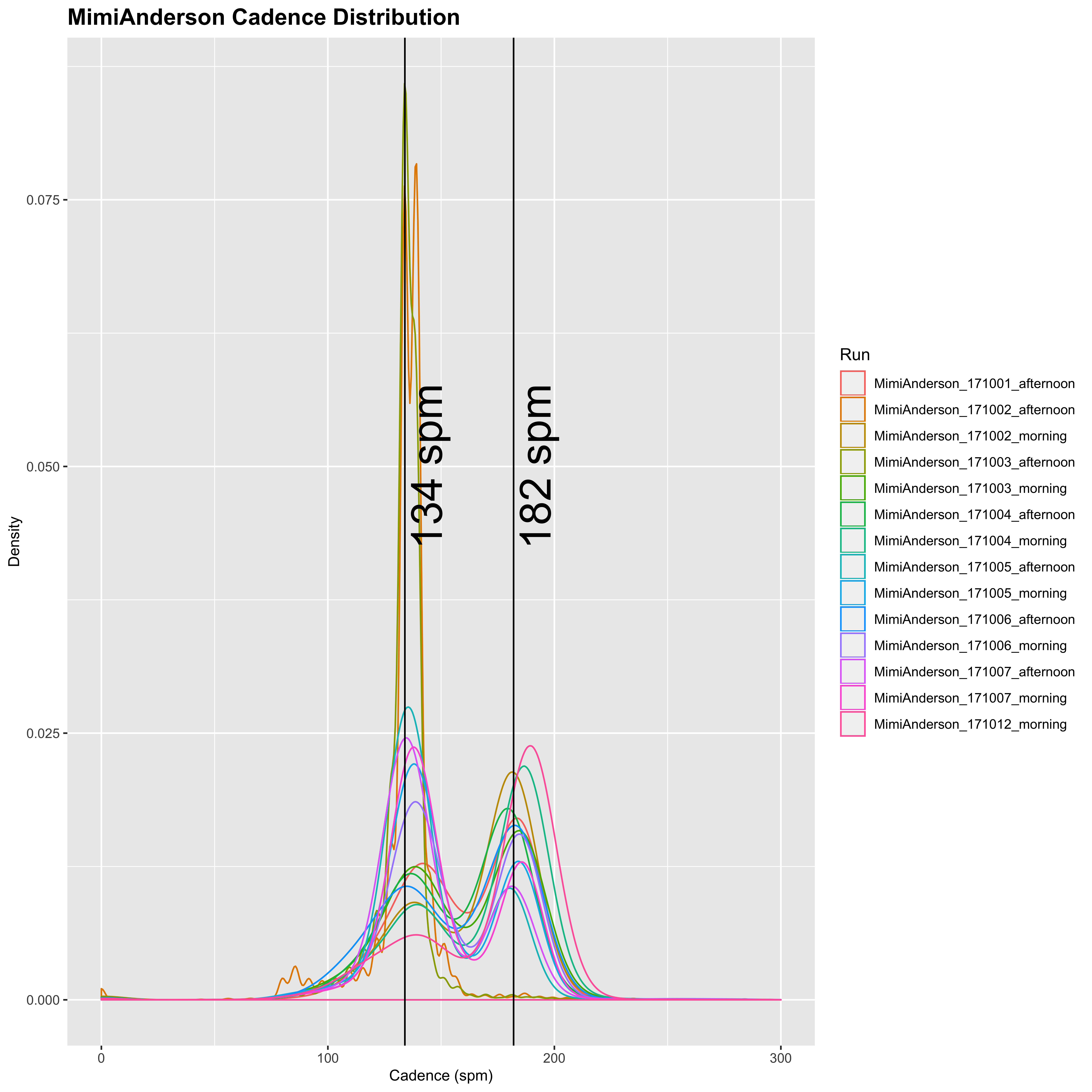

So Mimi runs with a cadence of around 134 spm for running and 182 spm for running. Now let’s look at Sandra’s:

plot_cadence_density("SandraVi")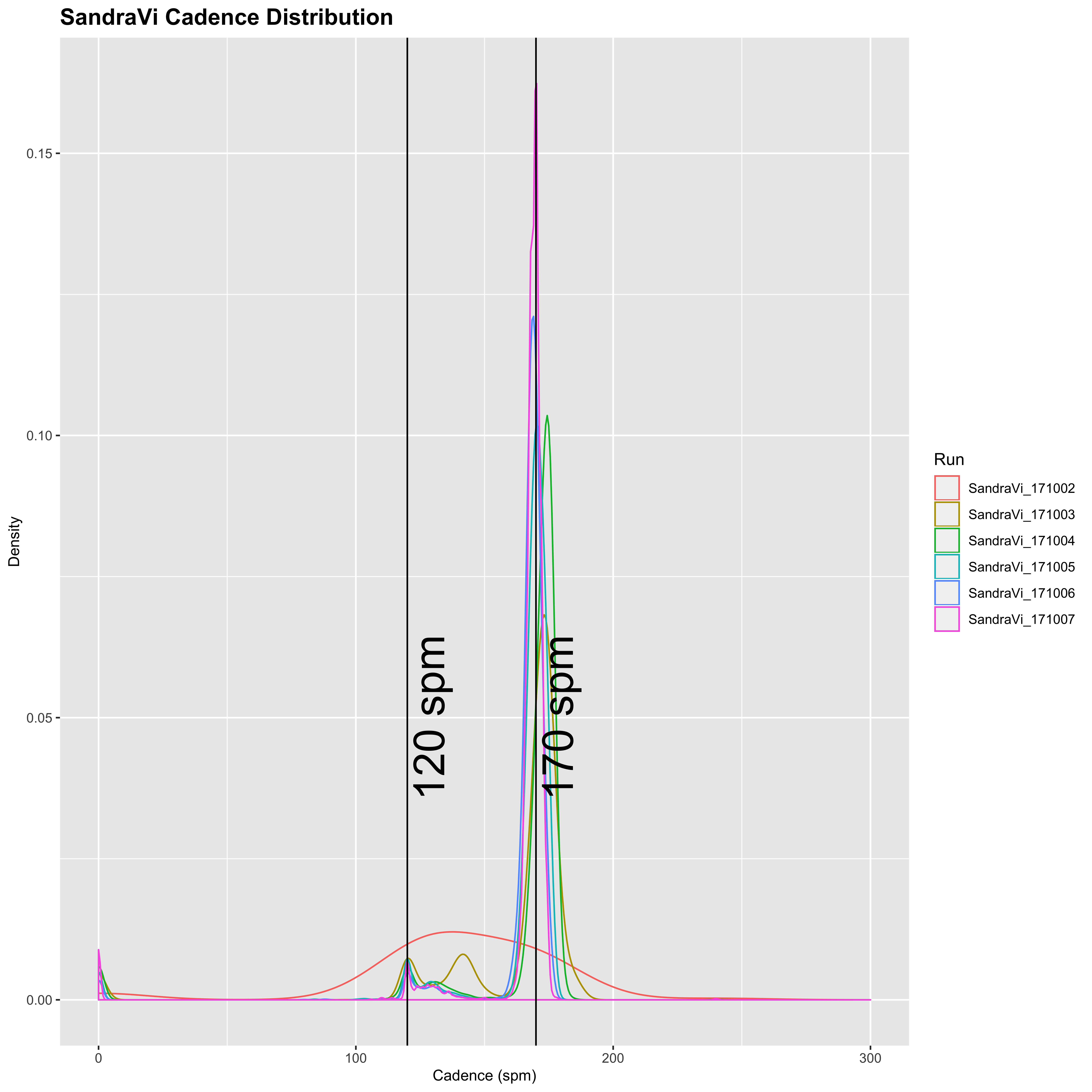

Sandra has generally lower cadence of 120 spm for walking, and 170 spm for running. She also appears from this to walk a lot less than Mimi, who seems to do a fairly even split between running and walking in general. In addition, the variation of Mimi’s running cadence is much higher than Sandra’s, so it appears that Sandra tends to run at a relatively constant cadence with a small amount of walking, whereas Mimi’s is much more variable and seems to be split in a 50:50 run/walk. Together with the longer differences between successive time-points, this may indicate that Sandra’s watch is set to pause automatically below a certain speed.

I also decided to look at my own data to see what that looked like:

plot_cadence_density("Mine")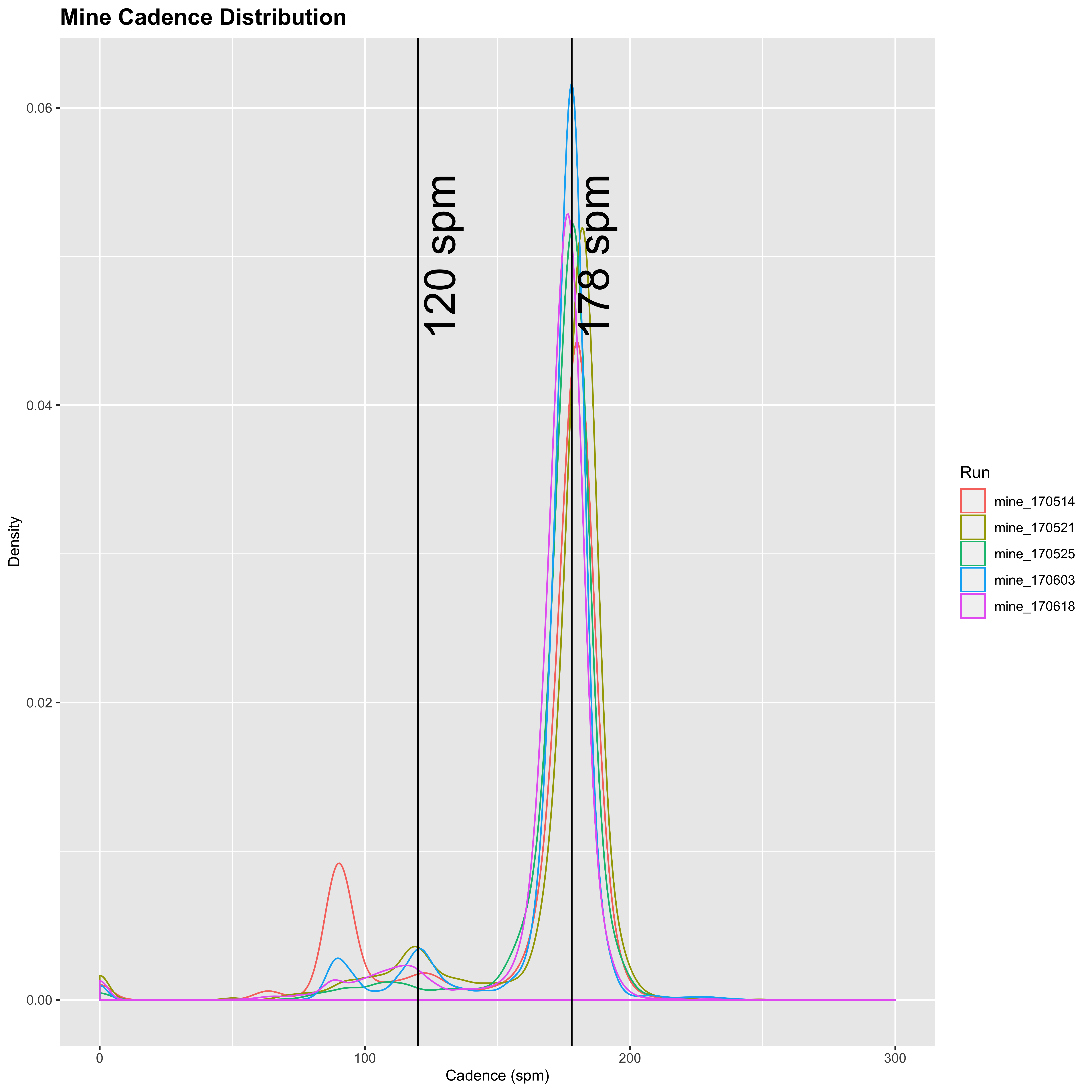

I also run with a fairly high cadence (just lower than Mimi’s but not dissimilar), and see more variation than Sandra. Now obviously I am not running across a continent in these runs - I am usually running with a belligerent dog who insists on stopping to sniff every bloody tree on the way. But it is not too dissimilar, and I see the distribution spreads out over 200 for some of the readings just like with Mimi. I’m an okay runner - probably not particularly good compared to many of the posters on LetsRun, but I do okay at shorter stuff and longer stuff. But it’s just a hobby for me, so I’m perfectly happy to self-associate as a hobby jogger. I don’t really know much about cadence, so I’m not sure if averaging 180+ is high or not? If nobody had suggested this was “garbage” and unbelievable, I would just assume that Mimi had a higher than normal cadence, similar to my own. I am a forefoot runner, and I think that Mimi is as well, and I believe that higher cadence tends to go hand in hand, but I am happy to bow to the experience of people more knowledgeable than myself in the matter.

To get an idea of the level of variation in the data (specifically the running cadence), let’s look at some aspects of that main distribution (excluding the outliers):

for (n in c("MimiAnderson", "SandraVi", "Mine")) {
  cad <- unlist(lapply(all_gpx[[n]], FUN = function (x) x[["extensions.cadence"]]))
  cad <- cad[cad > 150 & cad < 250]
  cat(sprintf("%12s: mode   = %d\n", n, Mode(cad)))
  cat(sprintf("%12s: mean   = %.2f\n", n, mean(cad)))
  cat(sprintf("%12s: median = %d\n", n, median(cad)))
  cat(sprintf("%12s: SD     = %.2f\n", n, sd(cad)))
  cat(sprintf("%12s: SEM    = %.3f\n", n, sd(cad)/sqrt(length(cad))))
  cat("\n")
}

MimiAnderson: mode = 182 MimiAnderson: mean = 181.56 MimiAnderson: median = 182 MimiAnderson: SD = 11.07 MimiAnderson: SEM = 0.026

SandraVi: mode   = 170
SandraVi: mean   = 171.13
SandraVi: median = 170
SandraVi: SD     = 4.54
SandraVi: SEM    = 0.029

    Mine: mode   = 178
    Mine: mean   = 177.96
    Mine: median = 178
    Mine: SD     = 7.53
    Mine: SEM    = 0.042

So clearly the standard deviation (SD) is much higher for Mimi’s data, but the standard error of the mean (SEM) is actually pretty comparable. SD and SEM, whilst both estimates of variability, tell you different things. The standard deviation is simply a measure of how different each individual data point is from the mean. It is descriptive of the data at hand. The SEM on the other hand is a measure of how far the mean of your sample is likely to be from the true population mean (under the assumption that each run is a random sampling of cadence values given Mimi’s true “normal” cadence). As your sample size increases, you more closely estimate the true mean of the population. This tells us that there is high variability in the sampling of cadence values for Mimi, but the precision is comparable with Sandra’s. This suggests nothing of whether the mean itself is actually believable of course, it is just worth noting the benefits of the increased sampling in these data.

So my overall feeling is that, whilst high, this was just the natural running gait of Mimi. Given recent events, this entire post ended up being highly expedited so that something was out there to provide a counter point to the accusations that have been made about data forgery and cheating, so in a rushed effort I looked around for some video of Mimi running to get an idea of her natural cadence. I found this video of her running at the end of her 7-day treadmill record. For the 18 seconds between 0:20 (when she begins to run properly) and 0:38 (when the camera pans away) I count 27-28 swings of her left hand/steps with her right foot, which would equate to a cadence of 180-187. Similarly, for the 16 seconds between 0:59 and 1:15, I count 24-25 swings/steps , which also equates to a cadence of 180-187. I’m not saying this is definitive proof, but this is at least evidence of her running with cadence similar to her average cadence across the USA, even at the end of 7 days on a treadmill. Adrenelin and a “sprint finish” mentality may play a role in achieving this as well of course. I would like to see more evidence of her running, and hopefully we will see some of that from the film crew that was with Mimi.

So here I have shown that, yes Mimi runs with a higher cadence than Sandra, but there is evidence that this is simply her natural gait. As to the fact that she regularly runs in the 185-195 range; well yes she does, but so do I. And I am no elite, particularly for these particular runs which are fairly perambulatory if I am honest. I can assure you that I have not doctored these data to be this mediocre. You can look through and even work out the points where my dog stopped to piss up a tree if you like. It’s not proof, but it is evidence.

I also wanted to look a bit into how the cadence actually corresponds to the speed at which the women are running. Below is a distribution plot showing the pace at each time point for each of the data sets considered here. Notice that I am excluding the data points where the runners are not moving to avoid divide by 0 errors in the pace calculation:

all_cor_dat <- list()
for (n in c("MimiAnderson", "SandraVi", "Mine", "Fake")) {
  cor_dat <- list()
  for (r in names(all_gpx[[n]])) {
    cor_dat[[r]]          <- all_gpx[[n]][[r]][,c("time.diff", "dist.travelled", "extensions.cadence")]
    cor_dat[[r]][["Run"]]  <- r
    cor_dat[[r]][["Pace"]] <- (cor_dat[[r]][["time.diff"]]/60)/(cor_dat[[r]][["dist.travelled"]])
  }
  cor_dat <- do.call(rbind.data.frame, cor_dat)
  cor_dat[["Name"]] <- n
  cor_dat           <- subset(cor_dat, dist.travelled != 0)
  all_cor_dat[[n]]  <- cor_dat
}
all_cor_dat <- do.call(rbind.data.frame, all_cor_dat)
ggplot(aes(x = Pace, color = Name), data = all_cor_dat) +
  geom_density(alpha = 0.25) +
  xlim(0, 20) +
  xlab("Pace (min/mile)") + 
  ylab("Density") +
  ggtitle("Pace Comparison Between Data Sets") +
  theme(axis.title = element_text(size = 10),
        plot.title = element_text(size = 15, face = "bold"))
## Warning: Removed 53290 rows containing non-finite values (stat_density).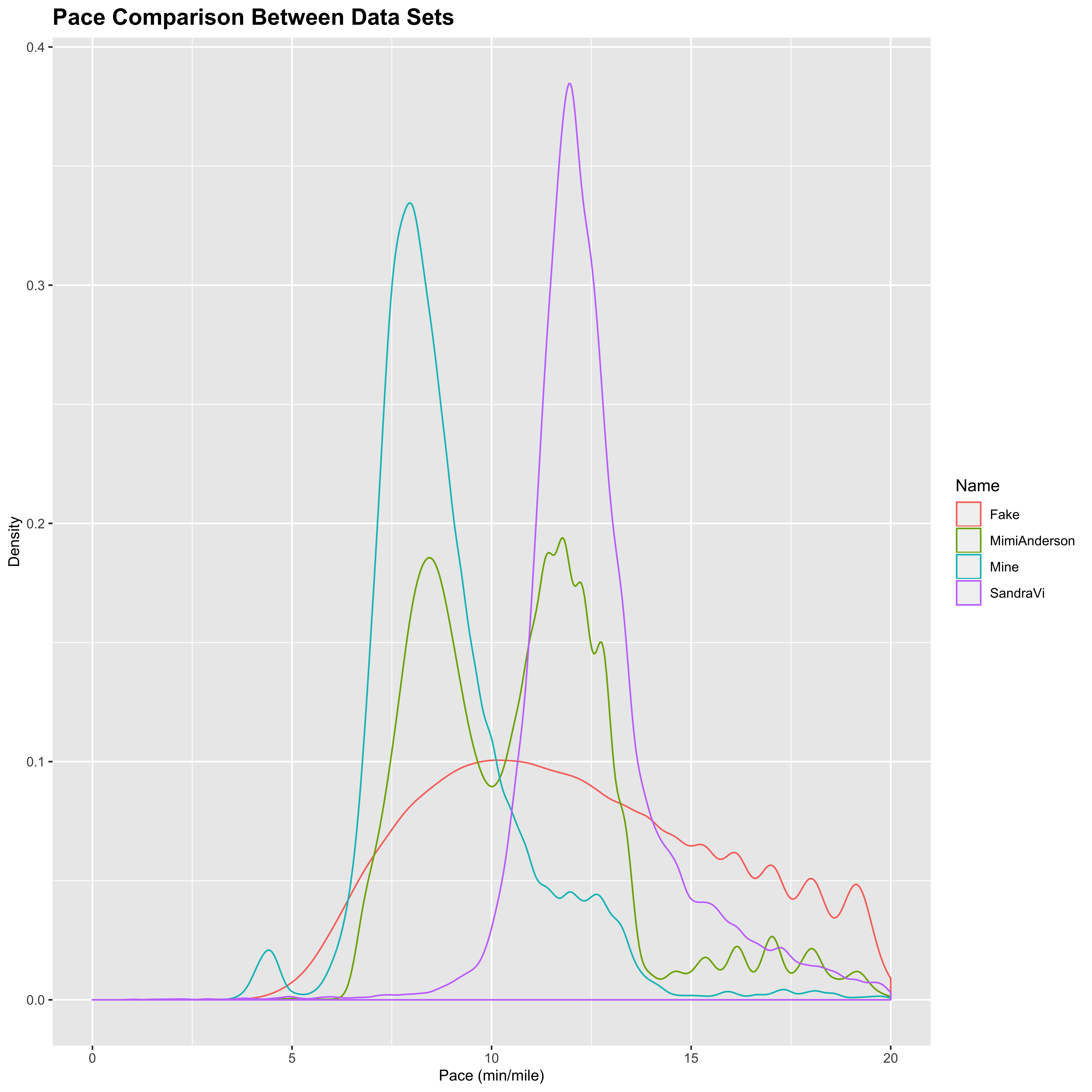

From this, we can see that there is a big difference in how the women are approaching the race. As noted before, Mimi runs in a fairly even 50:50 split of running and walking. This graph confirms that with a fairly even split between faster running of about 8.5 mins/mile and slower walking of about 11 mins/mile. Sandra on the other hand appears to be very steady in her approach, moving consistently at a 170 spm cadence run of about 11.5 mins/mile. This was earlier in the run and no doubt changed over time as Sandra began to close in on Mimi over the past week. My runs are predominantly spent jogging at around 8 mins/mile (with the occasional downhill thrown in for fun). The distribution for the fake data however does not follow the same type of distribution as the other runs (with a clearly delineated multimodal distribution for run/walk/sprint segments), and again stands out when compared with the ostensibly genuine data.

6.5 Spoofed data

So now I am getting to the nitty gritty of this post. The main accusation that I am attempting to quash is that of doctoring of the data. I have no answers regarding other perceived issues with the run, but the doctoring accusation I believe is a step too far. I have never denied that it would be possible to spoof the data. Of course it would. They are raw text files containing numbers - nothing more impressive than that. I did however think that spoofing it through Movescount would be very difficult, but it seems that I was wrong about that. It’s not simple to do, but it is doable with a little bit of know-how.

However, I do believe that it would be impossible to generate spoofed data that did not stand out as such when compared with genuine data. Faking data is notoriously hard. That’s not to say that people don’t do it all of the time, and sometimes it takes a while to pick up on. But I think that creating data out of thin air that also matched with what is going on with the tracker (I appreciate people have issues with the tracker, but I’m not getting into that), what is going on with reports from the crew, matched with environmental effects and the terrain that she was running over, what will ultimately come out from the film crew, and importantly what is self consistent, would be near impossible to manage. The cadence and times would have to make sense given the position, terrain and environmental effects into account. LetsRun user Scam_Watcheroo developed a tool to spoof the data, but he had the benefit of being able to track the things that might give the data away in advance. Mimi would have had to develop her method (or more accurately get somebody else to develop the method) blind, with no idea what sort of things might show it up as being faked. Sounds incredibly risky to me. So in thus section, I wanted to look at a few things to see if the different data sets stand up to scrutiny.

I am only touching the surface here, and I am looking into some more in depth methods to run statistical tests over the entire data set so far to check that the data are consistent and show the patterns one would expect. My hope in advance was that doing this would highlight the faked data as such. So to start with, I am not looking at consistency between the data sets, I am merely looking at the raw cadence data to look at a few potential things that might highlight anything that looked incongruous.

First of all I went back to simply looking at the time differences between the data points. For my data and Mimi’s data, they are almost all 1s differences, but there is the occasional blip (presumably when it is not able to update with the satellite straight away) leading to a few counts of around 2-7 secs. The spoofed data has none of these:

lapply(all_gpx[["Fake"]], FUN = function (x) table(x[["time.diff"]]))

$Fake_171001_afternoon

0     1 

25895 25894

$Fake_171002_afternoon

0     1 

26206 26205

$Fake_171002_morning

0     1 

29092 29091

$Fake_171007_afternoon

0     1 
1 19626 

$Fake_171007_morning

0     1 
1 27499 

The most recent ones (7th October) which were I think generated from scratch are ALL 1s differences, whilst the 2nd October ones (which were generated based on fiddling with Mimi’s uploads) were split half and half between 0s and 1s (a 0.5s sampling rate perhaps?). Either way, they do not have these little blips – the faked data appear to be too perfect. Being able to account for this and other such data imperfections heuristically (especially without knowing ahead of time that one would need to) would be bloody difficult and very very risky in my opinion.

I am also looking at how well the spoofed data stand up to scrutiny using some other methods. One obvious test would be to see whether the cadence data obey Benford’s Law, which shows that the first digits (and indeed second digits, third digits, etc.) have a unique logarithmic distribution such that smaller numbers are more likely than bigger numbers. Notice here that I am looking at half of the cadence, since the actual reported data in the .gpx file was doubled to give the cadence in spm. However, in this case the first digits are somewhat constrained, since the cadence is typically in a very narrow range resulting in a huge proportion of 8s and 9s:

n <- "Mine"
cad_dat <- list()
for (r in names(all_gpx[[n]])) {
  cad_dat[[r]] <- all_gpx[[n]][[r]][,c("name", "time", "extensions.cadence")]
  cad_dat[[r]][["Run"]] <- r
}
cad_dat <- do.call(rbind.data.frame, cad_dat)
cad_bentest <- benford(cad_dat[["extensions.cadence"]]/2, number.of.digits = 1)
plot(cad_bentest)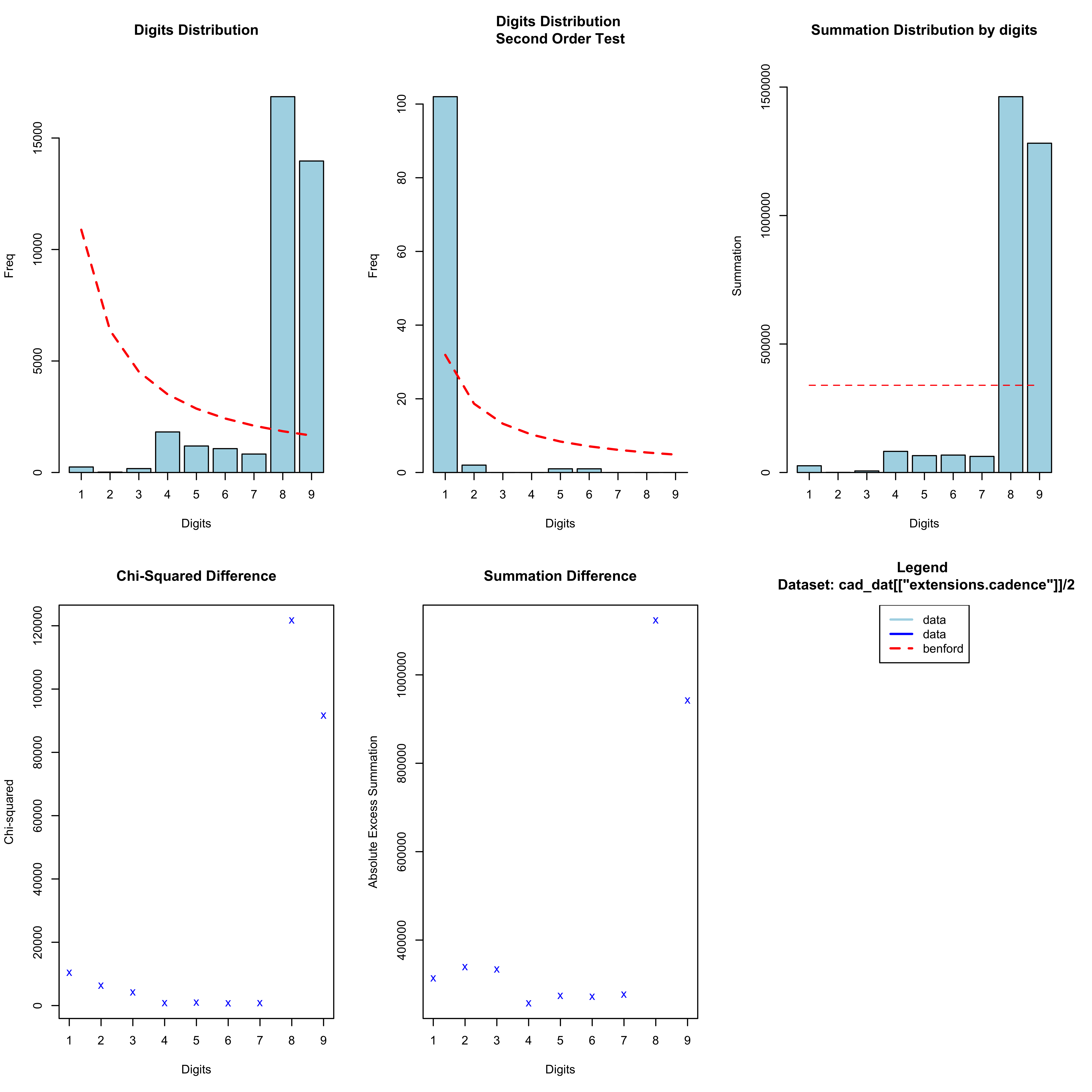

What about if we look at the second digit:

n <- "Mine"
cad_dat <- list()
for (r in names(all_gpx[[n]])) {
  cad_dat[[r]] <- all_gpx[[n]][[r]][,c("name", "time", "extensions.cadence")]
  cad_dat[[r]][["Run"]] <- r
}
cad_dat <- do.call(rbind.data.frame, cad_dat)
cad_bentest <- benford(as.numeric(substr(cad_dat[["extensions.cadence"]]/2, 2, 2)), number.of.digits = 1)
plot(cad_bentest)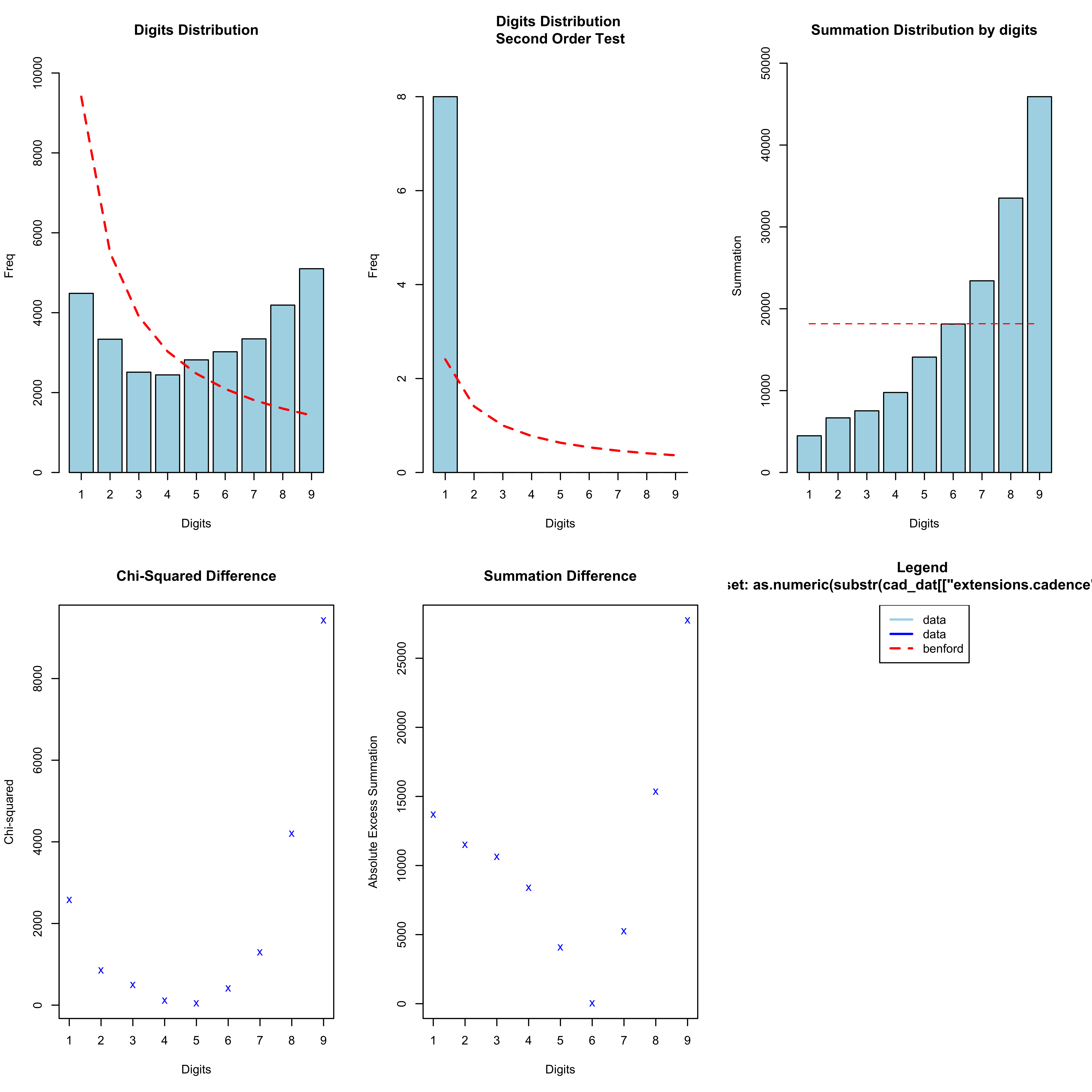

This is now approaching a more standardised distribution. It does not appear to follow Benford’s Law, but instead these data appear to be somewhat uniformly distributed. One idea that I have looked at is whether the trailing (and thus least significant) digits of the cadence data follow any particular distribution. Perhaps one might imagine that they should follow some distribution, such as the more uniform distribution seen above. Again remember here that I am plotting the raw cadence data, which is half of the cadence values reported in the distribution plots:

## Look at the final digit of the cadence data
all_digit_counts <- list()
all_digit_percent <- list()
for (n in names(all_gpx)) {
  all_digit <- matrix(0, ncol = 10, nrow = length(all_gpx[[n]]), dimnames = list(names(all_gpx[[n]]), as.character(0:9)))
  for (r in names(all_gpx[[n]])) {
      digit <- gsub("^\\d*(\\d)$", "\\1", all_gpx[[n]][[r]][["extensions.cadence"]]/2)
      all_digit[r, ] <- table(digit)[as.character(0:9)]
  }
  all_digit_counts[[n]]  <- all_digit
  all_digit_percent[[n]] <- 100*all_digit/rowSums(all_digit)
}
  
## Plot heatmap
hm_dat <- do.call(rbind.data.frame, all_digit_percent)
rownames(hm_dat) <- gsub("^.*\\.", "", rownames(hm_dat))
pheatmap(hm_dat, cluster_rows = FALSE, cluster_cols = FALSE, main = "Cadence - trailing digit percentage")#, display.numbers = FALSE,  annotation_legend = TRUE, cluster_cols = TRUE, show_colnames = TRUE, show_rownames = FALSE)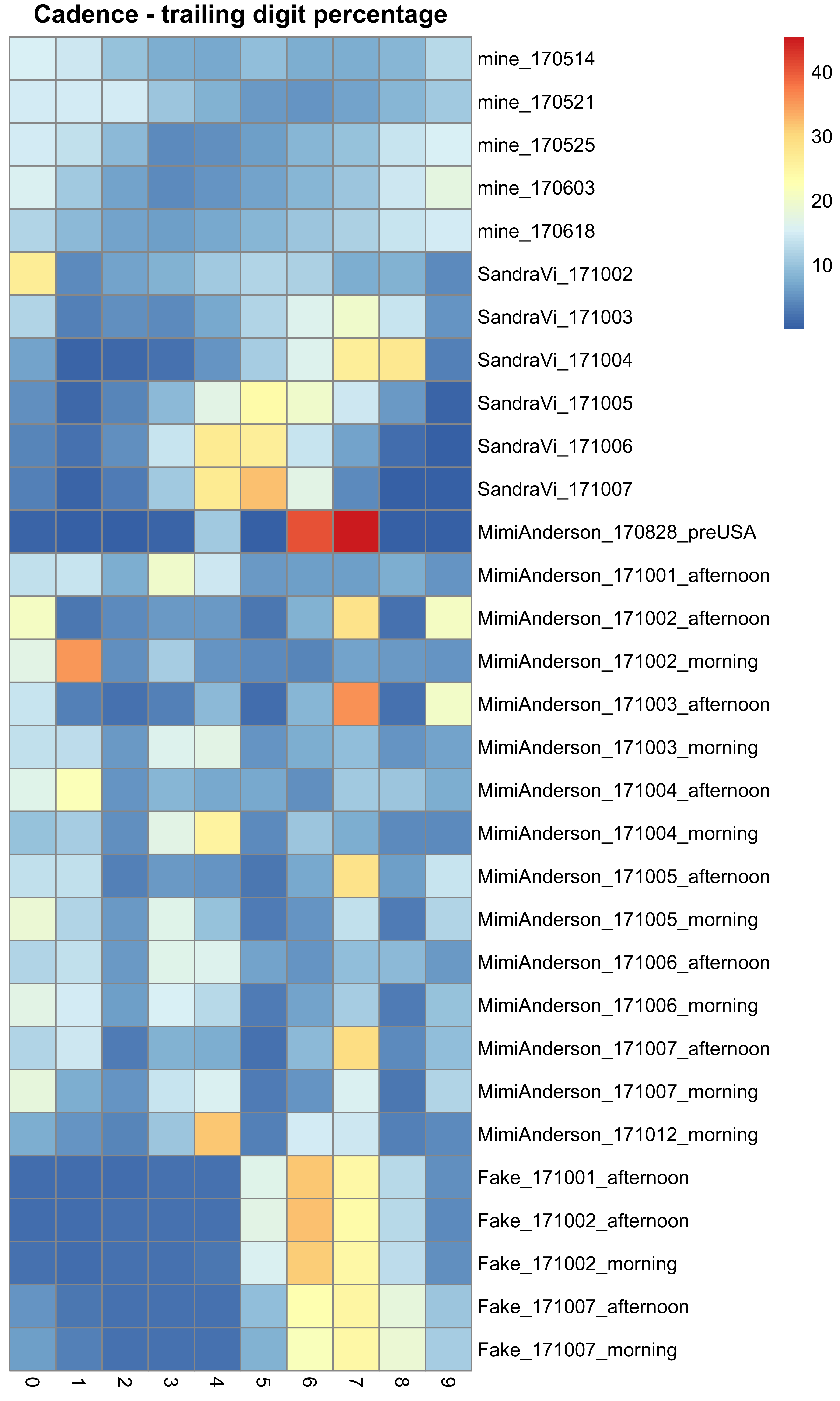

This figure shows the distribution of the percentage of trailing digits seen amongst the different data sets – Mimi’s, Sandra’s, the spoofed data, and some of my own runs. The colour of the heatmap indicates the percentage of times that digit is seen in the final position, with blue being less often and red being more often. In general:

• Mine seem to be quite uniformly distributed (mainly blue)
• Mimi’s are pretty uniform (except for the pre-USA run that I put in as well) with the exception of a regular depletion of 2s and 5s
• Sandra’s seem to show a depletion of 1s and 9s, and enrichment of several digits in most runs (but nothing consistent)
• The fake data however seem very consistent in their prevalence of 6s and 7s (and to a lesser extent 4s and 8s).

There is not really enough data here to identify a pattern, but from what is here the spoofed data stands out with a distribution that is different from that seen with my own data. Mimi’s is actually the most alike to data that I know to be real, although the depletion of certain digits is quite odd. But then the same is true for Sandra’s data as well to a greater degree (albeit different numbers). I plan to look into this in more detail using more data, including all of Sandra’s and Mimi’s runs, and a lot more genuine data taken from Strava as a base line to see if this distribution holds.

Obviously none of this “proves” these data are not fabricated. That is impossible. I do however thus far see no sufficient evidence to suggest that these data are not real (for both runners, although Sandra was never on “trial” here). And really I have only scratched the surface on how to test the validity of these data.