1 Introduction

Machine learning and artificial intelligence is a hot topic in the tech world, but the expression “machine learning” can describe anything from fitting a straight line through some data, to a machine able to think, learn and react to the world in highly sophisticated ways (e.g. self-driving cars if you want to be positive about AI, or SkyNet from Terminator if you want to be a naysayer). Whilst common machine learning techniques like support vector machines and k-Nearest Neighbour algorithms can be used to solve a huge number of problems, deep learning algorithms like neural networks are required to create these highly sophisticated models.

In this blog, I will explore the use of some commonly used tools for generating neural networks within the R programming language.

2 TensorFlow

TensorFlow is one of the most powerful tools for deep learning, and in particular is widely used for training neural networks to classify various aspects of images. It is a freely distributed open-source library in python (but mainly written in C++) originally created by Google, but has become the cornerstone of many deep learning models currently out there

A Tensor is a multi-dimensional array, and the TensorFlow libraries represent a highly efficient pipeline for the myriad linear algebra calculations required to generate new tensors through the layers of the network.

3 Keras

The Keras API is a high-level user-friendly neural network API (application programming interface) designed for accessing deep neural networks. One of the benefits is that it is able to run on GPUs as well as CPUs, which have been shown to work better for training neural networks since they are able more efficient at running the huge number of simple calculations required for model training (for example convolutions of image data).

Keras can be used an interface to TensorFlow for training deep multi-level networks for use in deep learning applications. Both are developed in python, but here I am going to use the RStudio interface to run a few simple deep learning models to trial the process ahead of a more in-depth application. R and python are somewhat at war in the data science community, with (in my opinion) R being better for more general data analysis and visualisation (for instance, whilst the python seaborn package produces beautiful images, the ggplot2 package is far more elaborate). However, with the Keras and TensorFlow packages (and the generally higher memory impact of using R), python is typically far more suited for deep learning applications.

However, the ability to access the Keras API through RStudio, and the amazing power of using RStudio to develop workflows, will make this a perfect “one stop shop” for data science needs. Much of this work is developed from the RStudio Keras and TensorFlow tutorials.

We first load the reticulate package to pipe python commands through R:

library("reticulate")

Then install and load the keras package. When we load it using the install_keras() function, we can define different backend engines and choose to use GPUs rather than CPUs, but for this example I will simply use the default TensorFlow backend on my laptop CPU:

devtools::install_github("rstudio/keras")
library("keras")

4 MNIST Database

So let’s have a little play by looking at a standard machine learning approach, looking at the MNIST dataset. This is the Modified National Institute of Standards and Technology database, and contains a large amount of images of handwritten digits that is used to train models for handwriting recognition. Ultimately, the same models can be used for a huge number of classification tasks.

mnist_dat <- dataset_mnist()

The dataset contains a training set of 60,000 images, and a test set of 10,000 images. Each image is pre-normalised such that each digit is a grayscale image that fits into a 28x28 pixel bounding box.Each image is also supplied with a label that tells us what the digit should really be. This dataset is commonly used as a kind of benchmark for new models, with people vying to build the model with the lowest error rate possible:

So let’s define our data sets. We will require two main data sets; a training set where we show the model the images and tell it what it should recognise, and a test dataset where we can predict the result and check against the ground level label. For each data set, we will create a dataset x containing all of the images, and a dataset y containing the labels:

training_dat_x_raw <- mnist_dat[["train"]][["x"]]
training_dat_y_raw <- mnist_dat[["train"]][["y"]]
test_dat_x_raw     <- mnist_dat[["test"]][["x"]]
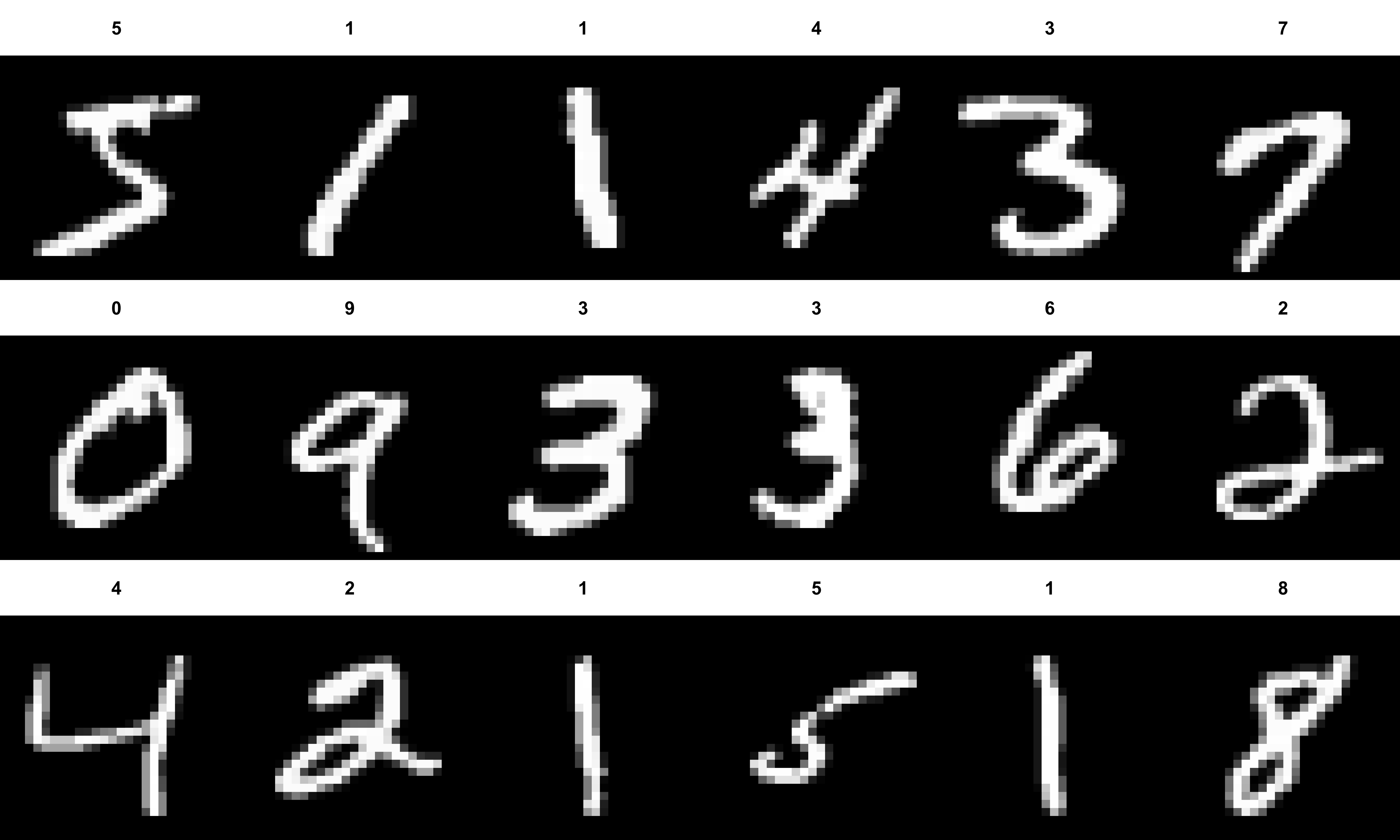
test_dat_y_raw     <- mnist_dat[["test"]][["y"]]

Each of the images is essentially a 2D array, with 28 rows and 28 columns, with each cell representing the greyscale value of the pixel. So the _dat_x data sets are 3D arrays. So accessing specific elements from these arrays in R is similar to accessing rows and columns using the [x,y] style axis, but we need to specify a third element z for the specific array that we want to access – [z,x,y]. So lets take a look at an exampl of the input data:

par(mfcol = c(3,6))
par(mar = c(0, 0, 3, 0), xaxs = 'i', yaxs = 'i')
for (i in 1:18) { 
  plot_dat <- training_dat_x_raw[i, , ]
  plot_dat <- t(apply(plot_dat, MAR = 2, rev)) 
  image(1:28, 1:28, plot_dat, 
        col  = gray((0:255)/255), 
        xaxt ='n', 
        main = training_dat_y_raw[i],
        cex  = 4, axes = FALSE)
}

5 Data Transformation

We can easily reduce this 3D data by essentially taking each 28x28 matrix and collapsing the 784 values down into a 1D vector. Then we can make one big 2D matrix containing all of the data. Ordinarily, this could be done by reassigning the dimensions of the array, but by using the array_reshape() function, the data is adjusted to meet the requirements for Keras:

training_dat_x <- array_reshape(training_dat_x_raw, c(nrow(training_dat_x_raw), 784))
test_dat_x     <- array_reshape(test_dat_x_raw,     c(nrow(test_dat_x_raw), 784))
dim(training_dat_x)

## [1] 60000   784

The values in these arrays are greyscale values, representing 256 integer values between 0 (black) and 255 (white). It will be useful for downstream analyses to rescale these values to real values in the range \([0,1]\):

training_dat_x <- training_dat_x/255
test_dat_x     <- test_dat_x/255

The R-specific way to deal with categorical data would be to encode the values in the y datasets to a factor with 10 levels (“0”, “1”, “2”, etc). However, Keras requires the data to be in a slightly different format, so we use the to_categorical() function instead. This will encode the value in a new matrix with 10 columns and n rows, such that every row contains exactly one 1 (representing the label) and nine 0s. This is known as an identity matrix. Keras uses a lot of linear algebra, and this encoding makes these calculations much simpler:

training_dat_y <- to_categorical(training_dat_y_raw, 10)
test_dat_y     <- to_categorical(test_dat_y_raw, 10)
dim(training_dat_y)

## [1] 60000    10

6 Sequential Models

A standard deep learning neural network model can be thought of as a number of sequential layers, with each layer representing a different abstraction of the data. For instance, consider a model looking at facial recognition from image data. The first layer might represent edges of different aspects of the image. The next layer might be designed to pick out nose shape. The next might pick out hair. The next might determine the orientation of the face. etc. Then by adding more and more layers, we can develop models able to classify samples based on a wide range of different features.

Of course, there is a danger in statistics of over-fitting data, which is when we create a model so specific for the training data that it becomes practically worthless. By definition, adding more variables into a model will always improve the fit, but at the cost of its applicability to other data sets. In models such as linear models, we look for parsimony – a model should be as complicated as it needs to be and no more complicated. The old phrase is:

When you hear hooves, think horse not zebra

However, deep learning sequential models such as these are robust to these problems, since model training can back-propagate, allowing us to incorporate far more levels than would be possible with other machine learning techniques.

The general steps involved in using Keras for deep learning are to first build your model, compile it to configure the parameters that will be used to develop the “best” model, train it using your training data, then test it on an additional data set to see how it copes.

So let’s build a simple sequential neural network model object using keras_model_sequential(), then add a series of additional layers that we hope will accurately identify our different categories. Adding sequential layers uses similar syntax to the tidyverse libraries such as dplyr, by using the pipe operator %>%:

model <- keras_model_sequential()
model %>%
  layer_dense(units = 28, input_shape = c(784)) %>%
  layer_activation(activation = "relu") %>%
  layer_dropout(rate = 0.4)

7 Dense Layer

The first layer is a densely connected neural network layer, which takes a set of nD input tensors (in this case 1D input tensors), and generate a weights matrix by breaking the tensor into subsets and using this to learn the weights by doing some linear algebra (vector and matrix multiplication). The output from the dense layer is then generated as follows:

\[output = activation(dot(input, kernel) + bias)\]

So the weights kernel is generated and multiplied (dot product) with the input. If requested, a bias is also calculated and added to account for any systematic bias identified in the data. An activation function is then used to generate the final tensor to go on to the following layer (in this case we have specified this is a separate layer).

8 Activation Layer

An activation function can often be necessary to ensure the back-propogation and gradient descent algorithms work. By default, no activation is used. However, this is a linear identity function, which is very limited. A common activation function is the Rectified Linear Unit (ReLU), which is linear for positive values, but zero for negative values. This is usually a good starting point as it is very simple and fast. Another option is the [softmax](https://en.wikipedia.org/wiki/Softmax_function) function, which transforms each input logit (the pre-activated values) by taking the exponential and normalizing by the sum of exponentials over all inputs so that the sum is exactly 1:

\[\sigma(y_i) = \frac{e^{y_i}}{\sum^{K}_{j=1}e^{y_j}}\]

It is commonly used for multinomial logistic regression, where a different softmax function is applied for each class with a different probability incorporated, since it is able to transform input numbers into probabilities. The use of exponentials ensures that there are no negative values, no matter how negative the input logit. So the softmax function outputs a probability distribution for potential outcomes in the range \([0,1]\).

9 Dropout Layer

Finally, we specify a dropout layer, which essentially drops a proportion of the nodes in the neural network to prevent over-fitting. In this case we have connections in the network between all of the tensor subsets generated. However, many of them are more useful in the model than others, so here we deactivate the 40% least useful nodes. Of course, this will reduce the training performance, but will prevent the issue of over-fitting making the model more generalised and applicable to other data sets. Model fitting is all about tweaking parameters and layers to get the most effective model, and this is one way in which we can improve the effectiveness of the model at predicting unseen data.

10 Define Initial Model

So let’s generate a more thorough model of 4 dense layers, gradually filtering down to a final output of 10 probabilities using the softmax activation function – the probabilities for the 10 digits:

MNIST_model <- keras_model_sequential()
MNIST_model %>%
  layer_dense(units = 256, input_shape = c(784)) %>%
  layer_activation(activation = "relu") %>%
  layer_dropout(rate = 0.4) %>%
  layer_dense(units = 128) %>%
  layer_activation(activation = "relu") %>%
  layer_dropout(rate = 0.3) %>%
  layer_dense(units = 56) %>%
  layer_activation(activation = "relu") %>%
  layer_dropout(rate = 0.2) %>%
  layer_dense(units = 10) %>%
  layer_activation(activation = "softmax")
summary(MNIST_model)

## Model: "sequential_1"
## ___________________________________________________________________________
## Layer (type)                     Output Shape                  Param #     
## ===========================================================================
## dense_1 (Dense)                  (None, 256)                   200960      
## ___________________________________________________________________________
## activation_1 (Activation)        (None, 256)                   0           
## ___________________________________________________________________________
## dropout_1 (Dropout)              (None, 256)                   0           
## ___________________________________________________________________________
## dense_2 (Dense)                  (None, 128)                   32896       
## ___________________________________________________________________________
## activation_2 (Activation)        (None, 128)                   0           
## ___________________________________________________________________________
## dropout_2 (Dropout)              (None, 128)                   0           
## ___________________________________________________________________________
## dense_3 (Dense)                  (None, 56)                    7224        
## ___________________________________________________________________________
## activation_3 (Activation)        (None, 56)                    0           
## ___________________________________________________________________________
## dropout_3 (Dropout)              (None, 56)                    0           
## ___________________________________________________________________________
## dense_4 (Dense)                  (None, 10)                    570         
## ___________________________________________________________________________
## activation_4 (Activation)        (None, 10)                    0           
## ===========================================================================
## Total params: 241,650
## Trainable params: 241,650
## Non-trainable params: 0
## ___________________________________________________________________________

Here we can see the change in shape of the tensors throughout the model, and the number of trainable parameters at each layer level. These are fully connected layers, so every neuron (values in the tensors) is connected to every other neuron. So the number of parameters (or connections) is given by multiplying the number of values in the input layer by the number in the previous layer plus one. So in total we have nearly a quarter of a million parameters to estimate here.

11 Compile Model

So next we can compile this model to tell it which methods we want to use to estimate these parameters:

MNIST_model %>% 
  compile(
    loss = "categorical_crossentropy",
    optimizer = optimizer_rmsprop(),
    metrics = c("accuracy")
  )

The loss function here is the method that will be used to optimise the parameters by comparing the predicted value with that of the actual value. Categorical crossentropy is commonly used in classification models when the output is a probability. It increases logarithmically as the predicted value diverges from the true value.

The optimizer is used to ensure that the algorithm converges in training. We are trying to minimise the loss function, so Gradient Descent can be used to optimse by iteratively recalculating the weights and bias until the minima is found. There is a danger of getting stuck at a local minima value, so sometimes it may be necessary to tune the parameters to avoid this. In this case, we are using RMSProp optimizer, which is similar to Gradient Descent but attempts to avoid this by adding oscillations to the descent.

Finally, we can specify which metrics we wish to output inorder to evaluate the model during training. Here we look at the accuracy to determine how often our model gives the correct prediction in the trained data.

12 Training the Model

So now let’s train our model with our training data to estimate the parameters:

training_output <- MNIST_model %>% 
  fit(
    training_dat_x, training_dat_y,
    batch_size = 128,
    epochs = 30,
    verbose = 1,
    validation_split = 0.2
  )

Here we are going to run the model using our reformated training data above. The epoch argument determines the number of iterations used to optimize the model parameters. In each epoch, we will use batch_size samples per epoch for the gradient update.

The validation_split argument is used for running cross-validation in order to evaluate the quality of the model. A portion of the training data is kept aside, and is used to validate the current model parameters and calculate the accuracy.

13 Results

Let’s take a look at how the accuracy and the loss (caluclated as categorical cross-entropy) change as the model training progresses:

plot(training_output)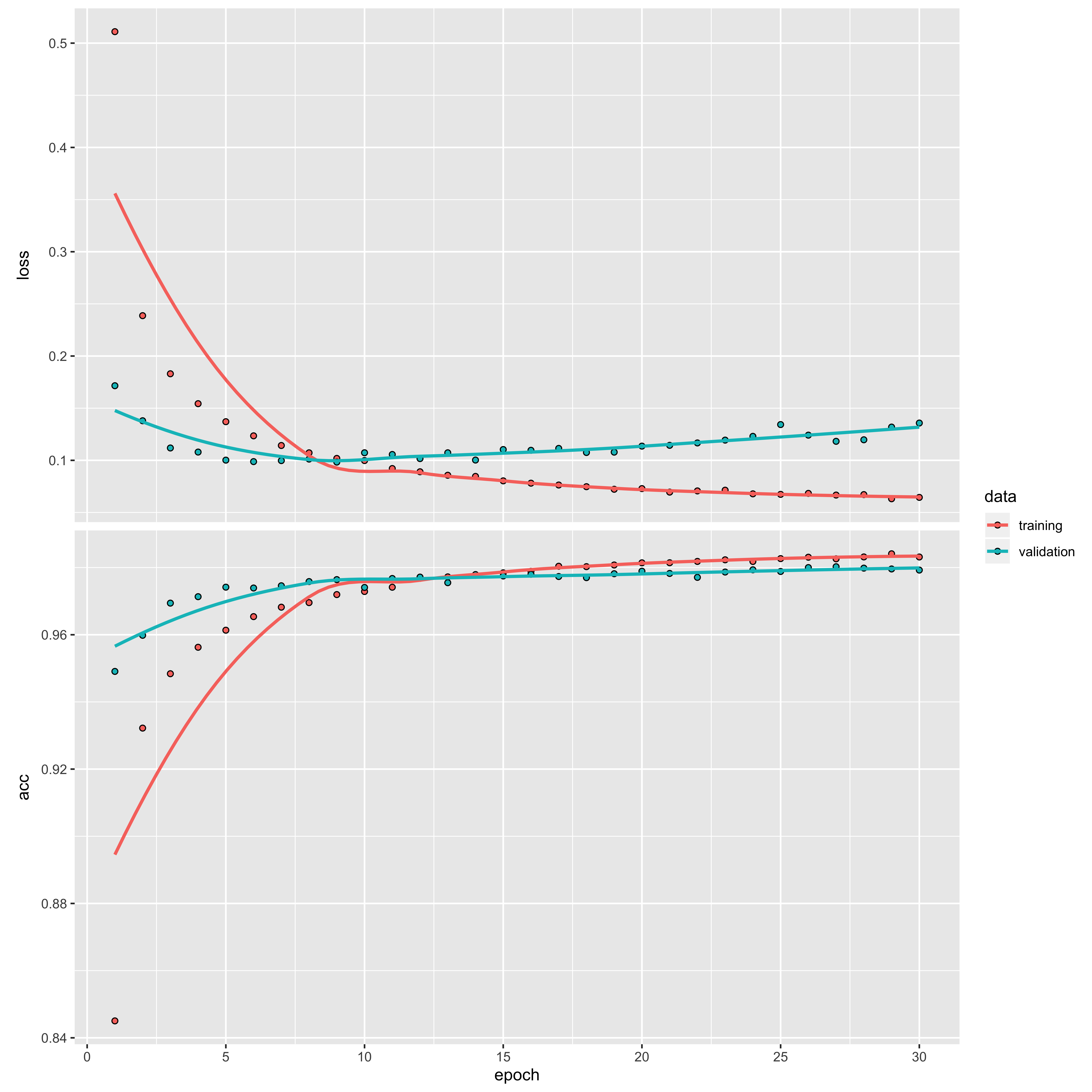

We can see that the loss is high and the accuracy low at the start of the training, but they quickly improve within the first 10 epochs. After this, they begin to plateau, resulting in a loss of 0.06 and accuracy of 98.31%.

This is pretty good, so let’s see how it works with the test set:

test_output <- MNIST_model %>% evaluate(test_dat_x, test_dat_y)
test_output

## $loss
## [1] 0.1132629
## 
## $acc
## [1] 0.9815

So 98.15% of the 10,000 test cases were predicted accurately. So this means that 185 were wrong. Let’s take a look at some of these:

predicted <- MNIST_model %>% predict_classes(test_dat_x)
which_wrong <- which(predicted != test_dat_y_raw)
par(mfcol = c(3,6))
par(mar = c(0, 0, 3, 0), xaxs = 'i', yaxs = 'i')
for (i in which_wrong[1:18]) {
  plot_dat <- test_dat_x_raw[i, , ]
  plot_dat <- t(apply(plot_dat, MAR = 2, rev)) 
  image(1:28, 1:28, plot_dat, 
        col  = gray((0:255)/255), 
        xaxt ='n', 
        main = paste("Predict =", predicted[i], "\nReal =", test_dat_y_raw[i]),
        cex  = 2, axes = FALSE)
}

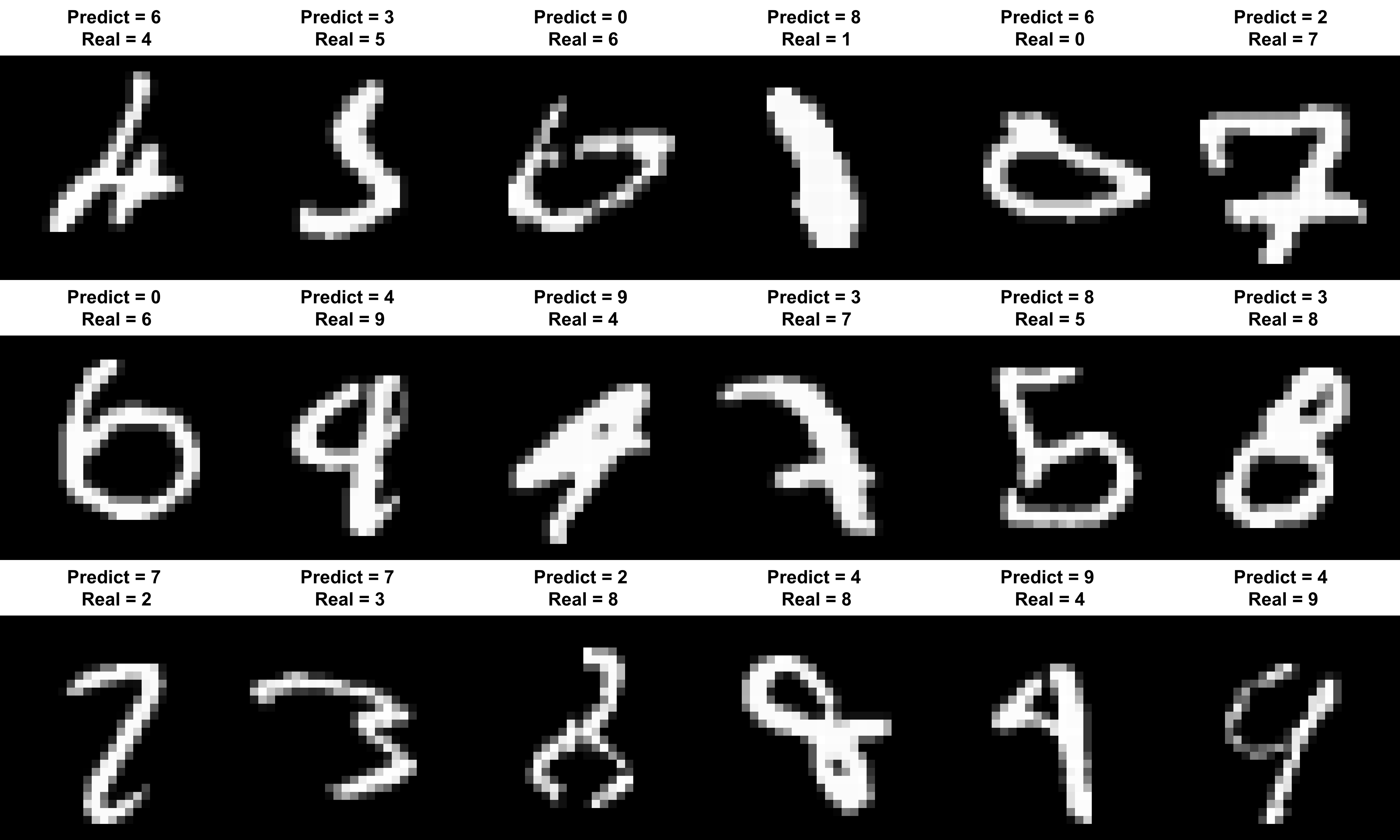
So we can see why the algorithm struggled with some of these, such as predicting 6s as 0s, and numbers that are slanted or squished. However, this obviously shows a lack of generalisation in the model, which is not brilliant for dealing with hand written numbers.

Obviously this is a fairly basic example of a neural network model, and the sorts of models being used in technology like self-driving cars contain far more layers than this. Model tuning is essential to compare and contrast models to identify the optimum model.

14 Conclusions

According to Wikipedia, one of the best results for the MNIST database used a hierarchical system of convolutional neural networks and managed to get an error rate of 0.23%. Here I have an error rate of 1.85%, so I clearly have a way to go! Often in classification algorithms, using standard machine learning algorithms will get you pretty far with pretty good error rates. However, to tune the models further to get error rates down to these sorts of levels, more complex models are required. Neural networks can be used to push the error rates down further. Getting the right answer 96% of the time is pretty good, but if you’re relying on that classification to tell whether there is a pedestrian stood in front of a self-driving car, it is incredibly important to ensure that this error rate is as close to 0 as possible.

However, this has been a very useful attempt at incorparting the powerful interface of Keras and the workflow of TensorFlow in R. Being able to incorporate powerful deep learning networks in R is incredobly useful, and will allow for incorporation with pre-existing pipelines already developed for bioinformatics analyses utilising the powerful pacakges available from Bioconductor.

Deep learning algorithms currently have a huge number of applications, from self-driving cars to facial recognition, and are being incorporated into technology in many industries. Development of deep learning algorithms and Big Data processing approaches will provide significant technological advancements. I am currently working on some potentially interesting applications, and hope to further my expertise in this area by working more with the R Keras API interface.

15 Session Info

sessionInfo()

## R version 3.6.1 (2019-07-05)
## Platform: x86_64-apple-darwin15.6.0 (64-bit)
## Running under: macOS Sierra 10.12.6
## 
## Matrix products: default
## BLAS:   /Library/Frameworks/R.framework/Versions/3.6/Resources/lib/libRblas.0.dylib
## LAPACK: /Library/Frameworks/R.framework/Versions/3.6/Resources/lib/libRlapack.dylib
## 
## locale:
## [1] en_GB.UTF-8/en_GB.UTF-8/en_GB.UTF-8/C/en_GB.UTF-8/en_GB.UTF-8
## 
## attached base packages:
## [1] stats     graphics  grDevices utils     datasets  methods   base     
## 
## other attached packages:
## [1] keras_2.2.5.0   reticulate_1.13
## 
## loaded via a namespace (and not attached):
##  [1] tidyselect_0.2.5  xfun_0.10         remotes_2.1.0    
##  [4] reshape2_1.4.3    purrr_0.3.3       lattice_0.20-38  
##  [7] colorspace_1.4-1  generics_0.0.2    testthat_2.2.1   
## [10] htmltools_0.4.0   usethis_1.5.1     yaml_2.2.0       
## [13] base64enc_0.1-3   rlang_0.4.1       pkgbuild_1.0.6   
## [16] pillar_1.4.2      glue_1.3.1        withr_2.1.2      
## [19] sessioninfo_1.1.1 plyr_1.8.4        tensorflow_2.0.0 
## [22] stringr_1.4.0     munsell_0.5.0     blogdown_0.16    
## [25] gtable_0.3.0      devtools_2.2.1    memoise_1.1.0    
## [28] evaluate_0.14     labeling_0.3      knitr_1.25       
## [31] callr_3.3.2       ps_1.3.0          tfruns_1.4       
## [34] curl_4.2          Rcpp_1.0.2        backports_1.1.5  
## [37] scales_1.0.0      desc_1.2.0        pkgload_1.0.2    
## [40] jsonlite_1.6      fs_1.3.1          ggplot2_3.2.1    
## [43] digest_0.6.22     stringi_1.4.3     dplyr_0.8.3      
## [46] bookdown_0.14     processx_3.4.1    grid_3.6.1       
## [49] rprojroot_1.3-2   cli_1.1.0         tools_3.6.1      
## [52] magrittr_1.5      tibble_2.1.3      lazyeval_0.2.2   
## [55] pkgconfig_2.0.3   crayon_1.3.4      whisker_0.4      
## [58] zeallot_0.1.0     ellipsis_0.3.0    Matrix_1.2-17    
## [61] prettyunits_1.0.2 assertthat_0.2.1  rmarkdown_1.16   
## [64] R6_2.4.0          compiler_3.6.1